modelling Level 4

Watershed Delineation and Flow Networks

Where does rainfall flow? Which streams feed this river? What area drains to this outlet? Watershed delineation extracts drainage basins from DEMs by tracing flow direction and accumulation. This model derives the D8 algorithm, implements pour point analysis, and extracts stream networks from terrain.

Prerequisites: flow direction, flow accumulation, basin extraction, graph traversal

27 Feb 2026 Updated 12 Mar 2026 17 min read

1. The Question

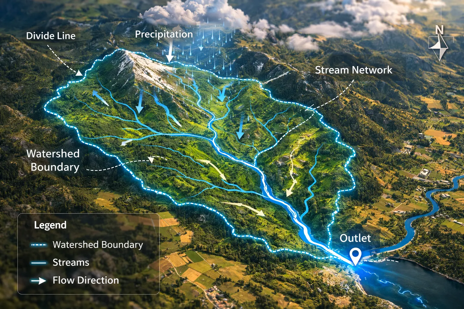
If it rains on this mountain, where does the water eventually flow?

Watershed (also called catchment or drainage basin): Area that drains to a common outlet.

Applications:

Flood prediction: How much area contributes flow to this point?
Water quality: Which land uses drain into this stream?
Reservoir planning: What’s the contributing area to a dam site?
Erosion modelling: Where does sediment originate and accumulate?
Ecological assessment: Upstream impacts on downstream habitats

The mathematical question: Given a DEM, how do we automatically extract:

Flow direction from each cell
Flow accumulation (contributing area)
Stream network (where flow accumulates)
Watershed boundaries for any pour point

2. The Conceptual Model

Flow Direction

Water flows downhill along path of steepest descent.

For each cell: Determine which neighbor receives flow.

D8 method (8-direction):

Examine all 8 neighbors
Flow to neighbor with steepest descent
Ties: Use deterministic rule (e.g., choose first in priority order)

Flow direction encoding:

64  128
[X]   1
 4    2

Powers of 2 → single value encodes direction.

Example: Flow to east (right) → direction = 1

Flow Accumulation

For each cell: Count how many upstream cells drain through it.

Algorithm:

Start with cells having no upstream contributors (ridges)
Process in topological order (high to low elevation)
Each cell passes its accumulated flow to its downstream neighbor

Result: Raster where value = number of contributing cells.

High accumulation = stream channels (many cells drain here)

Stream Network Extraction

Threshold accumulation to identify streams:

\[\text{stream} = (\text{accumulation} > T)\]

Typical threshold: T = 100-1000 cells (depends on DEM resolution)

Result: Binary raster of stream network.

Watershed Delineation

Pour point: Outlet location where we want to define watershed.

Watershed: All cells that drain to (flow through) pour point.

Algorithm: Trace upslope from pour point, marking all contributing cells.

3. Building the Mathematical Model

D8 Flow Direction

For cell at $(i, j)$ with elevation $z_{i,j}$:

Compute slope to each neighbor:

\[s_n = \frac{z_{i,j} - z_n}{d_n}\]

Where:

$z_n$ = elevation of neighbor
$d_n$ = distance to neighbor (1 for cardinal, $\sqrt{2}$ for diagonal)

Flow direction:

\[\text{dir}_{i,j} = \arg\max_n(s_n)\]

(Direction of maximum slope)

Edge cases:

Flat area ($s_n = 0$ for all neighbors):

Mark as undefined or use flat resolution algorithm

Depression (all neighbors higher):

Mark as sink or fill depression

Depression Filling

Depressions (local minima) disrupt flow routing.

Fill algorithm:

Initialize output DEM = input DEM
Set boundary cells to input elevation
Set interior cells to very high value
Iterate:
   - For each interior cell:
   - New elevation = min(current, max(neighbors) + epsilon)
Repeat until convergence

Result: DEM with depressions filled to spill elevation.

Epsilon (small value like 0.01m) ensures flow out of filled areas.

Flow Accumulation Algorithm

Pseudocode:

function flow_accumulation(flow_direction):
    # Initialize
    accumulation = ones(rows, cols)  # Each cell contributes itself
    
    # Sort cells by elevation (high to low)
    cells = sort_by_elevation_descending(DEM)
    
    # Process in topological order
    for each cell in cells:
        downstream = get_downstream_cell(cell, flow_direction)
        if downstream exists:
            accumulation[downstream] += accumulation[cell]
    
    return accumulation

Complexity: $O(n)$ after sorting $O(n \log n)$

Key: Topological ordering ensures upstream cells processed before downstream.

Watershed Extraction

Upslope area from pour point:

function extract_watershed(flow_direction, pour_point):
    watershed = empty_set()
    to_process = {pour_point}
    
    while to_process not empty:
        cell = to_process.pop()
        watershed.add(cell)
        
        # Find all neighbors that flow into this cell
        for each neighbor of cell:
            if flow_direction[neighbor] points to cell:
                to_process.add(neighbor)
    
    return watershed

Result: Set of all cells contributing flow to pour point.

4. Worked Example by Hand

Problem: Compute flow direction and accumulation for this DEM.

Elevation (meters):

      j=0  j=1  j=2  j=3
i=0    50   48   46   44
i=1    52   45   43   42
i=2    54   47   44   40
i=3    56   49   46   38

Use D8 method (8 neighbors).

Solution

Step 1: Flow Direction

Cell (0,1) elevation 48:

Neighbors and slopes:

(0,0): (48-50)/1 = -2 (uphill, ignore)
(0,2): (48-46)/1 = 2 ✓
(1,0): (48-52)/√2 = -2.83 (uphill)
(1,1): (48-45)/1 = 3 ✓
(1,2): (48-43)/√2 = 3.54 ✓ Maximum

Flow direction: Southeast diagonal (code = 2)

Cell (1,1) elevation 45:

Neighbors:

(0,0): -7/√2 (uphill)
(0,1): -3 (uphill)
(0,2): 2
(1,0): -7 (uphill)
(1,2): 2
(2,0): -9/√2 (uphill)
(2,1): -2 (uphill)
(2,2): 1

Maximum slope: (1,2) or (0,2) both = 2. Choose (1,2) by convention.

Flow direction: East (code = 1)

Continue for all cells…

Flow direction map:

      j=0  j=1  j=2  j=3
i=0     1    2    2    4
i=1     1    1    2    4
i=2     1    1    2    4
i=3     1    1    1    4

(1=E, 2=SE, 4=S)

Step 2: Flow Accumulation

Process cells in descending elevation order:

(3,0) elevation 56: Accumulation = 1, flows to (3,1)

Update (3,1): 1 + 1 = 2

(2,0) elevation 54: Accumulation = 1, flows to (2,1)

Update (2,1): 1 + 1 = 2

(1,0) elevation 52: Accumulation = 1, flows to (1,1)

Update (1,1): 1 + 1 = 2

(0,0) elevation 50: Accumulation = 1, flows to (0,1)

Update (0,1): 1 + 1 = 2

(3,1) elevation 49: Accumulation = 2, flows to (3,2)

Update (3,2): 1 + 2 = 3

Continue…

Final accumulation:

      j=0  j=1  j=2  j=3
i=0     1    2    4    8
i=1     1    2    5   10
i=2     1    2    6   13
i=3     1    2    3   16

Cell (3,3): Accumulates flow from all 16 cells (entire grid drains here).

This is the watershed outlet.

5. Computational Implementation

Below is an interactive watershed delineation tool.

Terrain type: Stream threshold: 50 cells Show flow direction: Show streams:

Click any cell to extract its watershed

Watershed area: -- cells

Max accumulation: -- cells

Try this:

Click right panel to set pour point (red dot) and extract watershed (green overlay)
Simple valley: Water flows down center channel
Ridge and valleys: Divides drainage into separate basins
Complex terrain: Multiple drainage patterns
Stream threshold: Higher = only major streams shown (blue)
Show flow direction: Red arrows show where each cell drains
Left: Elevation (lighter = higher)
Right: Flow accumulation (darker blue = more contributing area)

Key insight: Watershed boundaries follow ridges—all rain inside the green area flows to the red pour point!

6. Interpretation

Flood Risk Assessment

Contributing area = watershed size upstream of point.

Larger watershed → more runoff → higher flood potential

Example: Dam site with 500 km² watershed

Expected peak flow during storm
Reservoir sizing for flood control

Water Quality Management

Pollutant sources within watershed affect downstream quality.

Non-point source pollution:

Agricultural runoff (fertilizers, pesticides)
Urban stormwater (oil, sediment)
Septic systems

Delineate watershed → identify all potential sources → prioritize management.

Stream Order Classification

Strahler stream order:

First-order: Headwater streams (no tributaries)
Second-order: Junction of two first-order streams
Nth-order: Junction of two (n-1)-order streams

Higher order = larger river

Application: Stream classification for habitat assessment

Reservoir Yield

Runoff coefficient ($C$):

\[Q = C \times P \times A\]

Where:

$Q$ = runoff volume
$P$ = precipitation
$A$ = watershed area
$C$ = 0.1 (forest) to 0.9 (pavement)

Reservoir inflow = accumulated runoff from watershed

7. What Could Go Wrong?

Flat Areas

D8 fails where no downslope neighbor exists.

Solutions:

1. Impose flow direction:

Route to nearest definite flow (edge of flat)

2. D-infinity algorithm:

Allow fractional flow to multiple neighbors
More realistic but more complex

3. Epsilon slope:

Add tiny random elevation noise to break ties

Depressions and Sinks

Natural depressions:

Lakes (real features)
DEM artifacts (errors)

Consequences:

Flow accumulation terminates
Watershed extraction incomplete

Solutions:

Fill depressions:

Raise elevation to spill point
Loses lake information

Breach depressions:

Cut channel through lowest barrier
Preserves topography better

Hybrid:

Fill small artifacts, preserve large lakes

DEM Resolution

Coarse DEM misses small drainage features:

Ditches
Culverts
Small channels

Result: Incorrectly routed flow

Solution: Use finest available DEM (1m LiDAR ideal)

Edge Effects

Watershed extends beyond DEM boundary:

Flow direction undefined at edges.

Solution:

Use larger DEM extent
Or explicitly model boundary conditions

8. Extension: D-Infinity Algorithm

D8 limitation: Flow restricted to 8 directions (multiples of 45°).

D-infinity: Flow in any direction.

Method:

Fit plane to 3×3 neighborhood
Compute steepest descent direction (continuous)
Apportion flow to two nearest neighbors

Flow partitioning:

If steepest descent at angle $\theta$ between neighbors $A$ and $B$:

\[f_A = \frac{\theta_B - \theta}{\theta_B - \theta_A}\] \[f_B = 1 - f_A\]

Result: More realistic flow divergence

Cost: Higher computational complexity

9. Math Refresher: Topological Sorting

Definition

Topological sort: Linear ordering of directed acyclic graph (DAG) such that for every edge $u \to v$, $u$ comes before $v$ in the ordering.

Application to Flow

Flow network = DAG where edges point downstream.

Topological order = process cells from high to low elevation.

Ensures: When processing cell, all upstream contributors already processed.

Kahn’s Algorithm

L = empty list (topological order)
S = set of nodes with no incoming edges

while S not empty:
    remove node n from S
    add n to L
    for each node m with edge n → m:
        remove edge n → m
        if m has no other incoming edges:
            add m to S

For flow: Start with ridge cells (no upstream), process downhill.

Elevation Sorting

Simpler for DEMs: Sort by elevation instead of graph structure.

Works because: Higher elevation → upstream in flow network.

Summary

Watershed (drainage basin) = area that drains to a common outlet
D8 algorithm computes flow direction from each cell to steepest neighbor
Flow accumulation counts upstream contributing cells by processing in elevation order
Stream network extracted by thresholding flow accumulation (>100-1000 cells)
Watershed delineation traces upslope from pour point to find all contributors
Depression filling removes artificial sinks before flow routing
Applications: Flood risk, water quality, reservoir planning, erosion modelling
Challenges: Flat areas, depressions, DEM resolution, edge effects
D-infinity extends to continuous flow direction (more realistic, more complex)
Critical for hydrological modelling and environmental management