Vegetation Indices and Remote Sensing
Vegetation reflects near-infrared light strongly but absorbs red light (for photosynthesis). This spectral signature enables satellites to map greenness globally. This model derives NDVI and EVI, explains why they correlate with photosynthesis, and shows how to interpret vegetation index time series.
Prerequisites: spectral indices, normalized difference, reflectance, band ratios
1. The Question
How do satellites measure plant health and productivity from space?
From 700 km overhead, satellites observe Earth in multiple wavelengths (colors). Healthy vegetation has a distinctive spectral signature:
- Red light (620–700 nm): Strongly absorbed by chlorophyll → low reflectance (~5–10%)
- Near-infrared (NIR, 780–900 nm): Strongly reflected by leaf structure → high reflectance (~40–50%)
This contrast creates vegetation indices—mathematical combinations of spectral bands that quantify “greenness” and correlate with:
- Leaf area index (LAI)
- Photosynthesis rate (GPP from Model 20)
- Biomass
- Crop yield
The mathematical question: How do we combine red and NIR reflectance to create a robust vegetation index?
2. The Conceptual Model
Spectral Reflectance
Reflectance ($\rho$) is the fraction of incident light reflected by a surface:
\[\rho_{\lambda} = \frac{E_{\text{reflected}}(\lambda)}{E_{\text{incident}}(\lambda)}\]Where $\lambda$ is wavelength.
Typical vegetation reflectance:
- Blue (450–500 nm): Low (~5%, absorbed by chlorophyll)
- Green (500–580 nm): Moderate (~10%, why leaves look green)
- Red (620–700 nm): Very low (~5%, strong chlorophyll absorption)
- NIR (780–900 nm): High (~40–50%, internal leaf structure scattering)
- SWIR (1550–1750 nm): Low (~10–20%, water absorption)
Why NIR is High for Vegetation
Leaf internal structure:
- Spongy mesophyll: Air-cell interfaces scatter light
- Minimal absorption: No chlorophyll in NIR
- Result: Multiple scattering → high reflectance
Senescent leaves (dying, autumn colors):
- Chlorophyll breaks down
- Red reflectance increases (~20–30%)
- NIR decreases (~30–40%)
- Red-NIR contrast weakens → lower vegetation index
Soil Background
Bare soil has:
- Similar red and NIR (~15–25% both)
- Low red-NIR contrast
- Low vegetation index (as expected)
Partial cover: Mixture of vegetation and soil → intermediate index.
3. Building the Mathematical Model
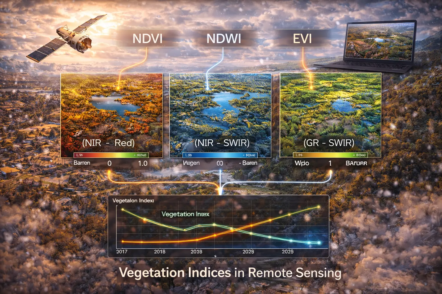
Normalized Difference Vegetation Index (NDVI)
The most widely used vegetation index:
\[\text{NDVI} = \frac{\rho_{\text{NIR}} - \rho_{\text{red}}}{\rho_{\text{NIR}} + \rho_{\text{red}}}\]Properties:
- Range: −1 to +1
- Dense vegetation: NDVI ≈ 0.7–0.9 (high NIR, low red)
- Sparse vegetation: NDVI ≈ 0.2–0.5
- Bare soil: NDVI ≈ 0.05–0.2
- Water: NDVI ≈ −0.1 to 0 (NIR absorbed by water)
- Clouds/snow: NDVI ≈ 0 to 0.3 (both red and NIR high and similar)
Why normalize?
- Reduces effects of illumination angle
- Reduces atmospheric scattering
- Makes values comparable across scenes
Enhanced Vegetation Index (EVI)
EVI reduces sensitivity to soil and atmosphere:
\[\text{EVI} = G \frac{\rho_{\text{NIR}} - \rho_{\text{red}}}{\rho_{\text{NIR}} + C_1 \rho_{\text{red}} - C_2 \rho_{\text{blue}} + L}\]Where:
- $G = 2.5$ (gain factor)
- $C_1 = 6$, $C_2 = 7.5$ (coefficients for atmospheric correction)
- $L = 1$ (soil adjustment factor)
Advantages over NDVI:
- Less saturated at high LAI
- Better atmospheric correction
- Improved sensitivity in dense canopies
MODIS EVI uses these exact coefficients.
Simple Ratio (SR)
The simple ratio predates NDVI:
\[\text{SR} = \frac{\rho_{\text{NIR}}}{\rho_{\text{red}}}\]Properties:
- Range: 0 to ~30
- Dense vegetation: SR ≈ 8–15
- Bare soil: SR ≈ 1–2
Relationship to NDVI:
\[\text{NDVI} = \frac{\text{SR} - 1}{\text{SR} + 1}\]SR has larger dynamic range but is more sensitive to noise.
Connecting to Leaf Area Index
Empirical relationship:
\[\text{LAI} \approx a \times \text{NDVI}^b\]Or approximately linear for moderate LAI:
\[\text{LAI} \approx 6 \times \text{NDVI}\]Saturation: At high LAI (> 5), NDVI saturates (approaches 0.9 asymptotically). EVI remains more responsive.
Connecting to Photosynthesis
fPAR (fraction of Photosynthetically Active Radiation absorbed):
\[\text{fPAR} \approx 1.24 \times \text{NDVI} - 0.168\](For NDVI between 0.15 and 0.9)
GPP estimation:
\[\text{GPP} \approx \varepsilon \times \text{fPAR} \times \text{PAR}\]Where:
- $\varepsilon$ = light use efficiency (~1–2 g C/MJ PAR)
- PAR = photosynthetically active radiation (from solar radiation measurements)
This is the basis for MODIS GPP product.
4. Worked Example by Hand
Problem: A Landsat scene has the following reflectance values for a pixel:
- Red: $\rho_{\text{red}} = 0.08$
- NIR: $\rho_{\text{NIR}} = 0.42$
- Blue: $\rho_{\text{blue}} = 0.06$
Calculate:
(a) NDVI
(b) Simple Ratio (SR)
(c) EVI
(d) Estimated LAI
Solution
(a) NDVI
\[\text{NDVI} = \frac{\rho_{\text{NIR}} - \rho_{\text{red}}}{\rho_{\text{NIR}} + \rho_{\text{red}}} = \frac{0.42 - 0.08}{0.42 + 0.08}\] \[= \frac{0.34}{0.50} = 0.68\](b) Simple Ratio
\[\text{SR} = \frac{\rho_{\text{NIR}}}{\rho_{\text{red}}} = \frac{0.42}{0.08} = 5.25\]Check relationship:
\(\text{NDVI} = \frac{SR - 1}{SR + 1} = \frac{5.25 - 1}{5.25 + 1} = \frac{4.25}{6.25} = 0.68\) ✓
(c) EVI
\[\text{EVI} = 2.5 \frac{0.42 - 0.08}{0.42 + 6(0.08) - 7.5(0.06) + 1}\] \[= 2.5 \frac{0.34}{0.42 + 0.48 - 0.45 + 1}\] \[= 2.5 \frac{0.34}{1.45} = 2.5 \times 0.234 = 0.59\](d) Estimated LAI
\[\text{LAI} \approx 6 \times \text{NDVI} = 6 \times 0.68 = 4.08\]Interpretation: NDVI = 0.68 indicates healthy, moderately dense vegetation (corn mid-season, temperate forest canopy). LAI ≈ 4 is typical for mature crops.
5. Computational Implementation
Below is an interactive vegetation index calculator with spectral reflectance curves.
NDVI:
EVI:
Simple Ratio:
Est. LAI:
Classification:
Try this:
- Dense vegetation: High NIR peak (~850 nm), low red trough → high NDVI
- Bare soil: Similar red and NIR → low NDVI (~0.1–0.2)
- Water: Very low NIR absorption → negative NDVI
- Snow: High reflectance across all bands → NDVI near zero
- Notice: The “red edge” (sharp increase 700–750 nm) is characteristic of vegetation
Key insight: The red-NIR contrast uniquely identifies photosynthetically active vegetation.
6. Interpretation
Seasonal Patterns
NDVI time series tracks growing season:
- Spring: NDVI rises (green-up, leaf emergence)
- Summer: NDVI peaks (maximum LAI)
- Autumn: NDVI declines (senescence, leaf fall)
- Winter: NDVI low (dormancy, snow cover)
Example: Temperate deciduous forest:
- January: NDVI ≈ 0.2 (bare branches)
- July: NDVI ≈ 0.8 (full canopy)
Drought Detection
Water stress reduces:
- Leaf area (wilting, leaf drop)
- Chlorophyll content
- NIR reflectance (leaf structure degrades)
Result: NDVI declines during drought.
Agricultural monitoring: Compare current NDVI to historical average → detect crop stress.
Global Patterns
NDVI maps reveal:
- Tropical rainforests: NDVI > 0.8 year-round
- Savannas: Seasonal variation (0.3–0.7)
- Deserts: NDVI < 0.2
- Tundra: Brief summer peak (0.3–0.5)
- Croplands: Strong seasonal cycle
MODIS NDVI (500 m resolution, 16-day) is the standard global product.
7. What Could Go Wrong?
Atmospheric Contamination
Aerosols and water vapor scatter blue/red more than NIR:
- Increases apparent NIR
- Decreases apparent red
- Inflates NDVI
Mitigation:
- Atmospheric correction (6S model, dark object subtraction)
- EVI includes blue band for correction
- Use imagery from clear days
Soil Background
In sparse vegetation, soil dominates signal:
- Bright soil → high reflectance in all bands
- Dark soil → low reflectance
Soil-Adjusted Vegetation Index (SAVI):
\[\text{SAVI} = \frac{(1 + L)(\rho_{\text{NIR}} - \rho_{\text{red}})}{\rho_{\text{NIR}} + \rho_{\text{red}} + L}\]Where $L = 0.5$ for moderate cover (adjust 0–1 based on density).
Saturation at High LAI
NDVI saturates when LAI > 5:
- Forest canopies (LAI = 6–8) all have NDVI ≈ 0.85–0.90
- Cannot distinguish between mature forest and very dense forest
Solution: Use EVI (less saturation) or NIRv (NIR × NDVI).
Confusing NDVI with Biomass
NDVI ∝ LAI (leaf area), not total biomass.
A grassland with LAI = 4 has similar NDVI to a forest with LAI = 4, but the forest has 100× more biomass (wood).
For biomass: Use SAR (Synthetic Aperture Radar) or LiDAR.
8. Extension: Other Vegetation Indices
Normalized Difference Water Index (NDWI):
\[\text{NDWI} = \frac{\rho_{\text{NIR}} - \rho_{\text{SWIR}}}{\rho_{\text{NIR}} + \rho_{\text{SWIR}}}\]Sensitive to water content in vegetation (drought stress).
Chlorophyll Indices:
- Use red edge (705–750 nm) for chlorophyll content
- More sensitive to plant health than NDVI
Photochemical Reflectance Index (PRI):
\[\text{PRI} = \frac{\rho_{531} - \rho_{570}}{\rho_{531} + \rho_{570}}\]Tracks xanthophyll cycle → photosynthetic light use efficiency.
9. Math Refresher: Normalization and Indices
Why Normalize?
Problem: Reflectance values change with:
- Illumination angle (sun elevation)
- Atmospheric conditions
- Sensor calibration
Solution: Normalize by forming ratios.
Example: Instead of $\rho_{\text{NIR}} - \rho_{\text{red}}$, use:
\[\text{NDVI} = \frac{\rho_{\text{NIR}} - \rho_{\text{red}}}{\rho_{\text{NIR}} + \rho_{\text{red}}}\]Effect:
- Range: Always −1 to +1
- Insensitive to uniform brightness changes
- Comparable across scenes
Index Properties
Symmetric indices:
$f(a, b) = -f(b, a)$
Example: NDVI$(b, a) = -$NDVI$(a, b)$
Bounded:
Output constrained to known range (e.g., −1 to 1)
Monotonic:
Increases with target variable (e.g., NDVI increases with LAI)
Summary
- NDVI = $(NIR - Red) / (NIR + Red)$: Most common vegetation index
- Range: −1 (water) to +1 (dense vegetation)
- Dense vegetation: NDVI ≈ 0.7–0.9 (high NIR, low red)
- Bare soil: NDVI ≈ 0.1–0.2 (similar red and NIR)
- EVI improves on NDVI for dense canopies and atmospheric effects
- Simple Ratio (NIR/Red) has larger dynamic range but more noise
- NDVI correlates with LAI, fPAR, and GPP
- Seasonal NDVI tracks growing season (green-up, peak, senescence)
- Red edge (700–750 nm) is diagnostic of healthy vegetation
- Vegetation indices enable global monitoring of photosynthesis from space