modelling Level 3

Snow Water Equivalent Estimation

How do we measure snow water equivalent across mountain basins? Ground observations (SNOTEL, snow courses) provide point measurements. Remote sensing (passive microwave, LiDAR) enables spatial coverage. This model derives microwave emission theory, implements snow depth-to-SWE conversion, and combines multi-sensor observations to map snowpack water content.

Prerequisites: microwave radiometry, snow depth density, sensor integration, uncertainty propagation

27 Feb 2026 Updated 12 Mar 2026 12 min read

1. The Question

What’s the total water stored in snow across a 1000 km² mountain basin?

Three measurement approaches:

1. Ground observations (point data):

SNOTEL stations (automated)
Manual snow courses (monthly surveys)
Snow pillows (weight measurement)

2. Remote sensing (spatial coverage):

Passive microwave (AMSR-E, SSMIS)
Active microwave (SAR)
LiDAR (airborne snow depth)
Optical (MODIS snow cover extent)

3. Model-data fusion:

Combine observations with snow models
Assimilation techniques
Produce gridded SWE estimates

The mathematical question: How do we convert different measurements (microwave brightness temperature, snow depth, weight) into SWE, and how do we scale from points to basins?

2. The Conceptual Model

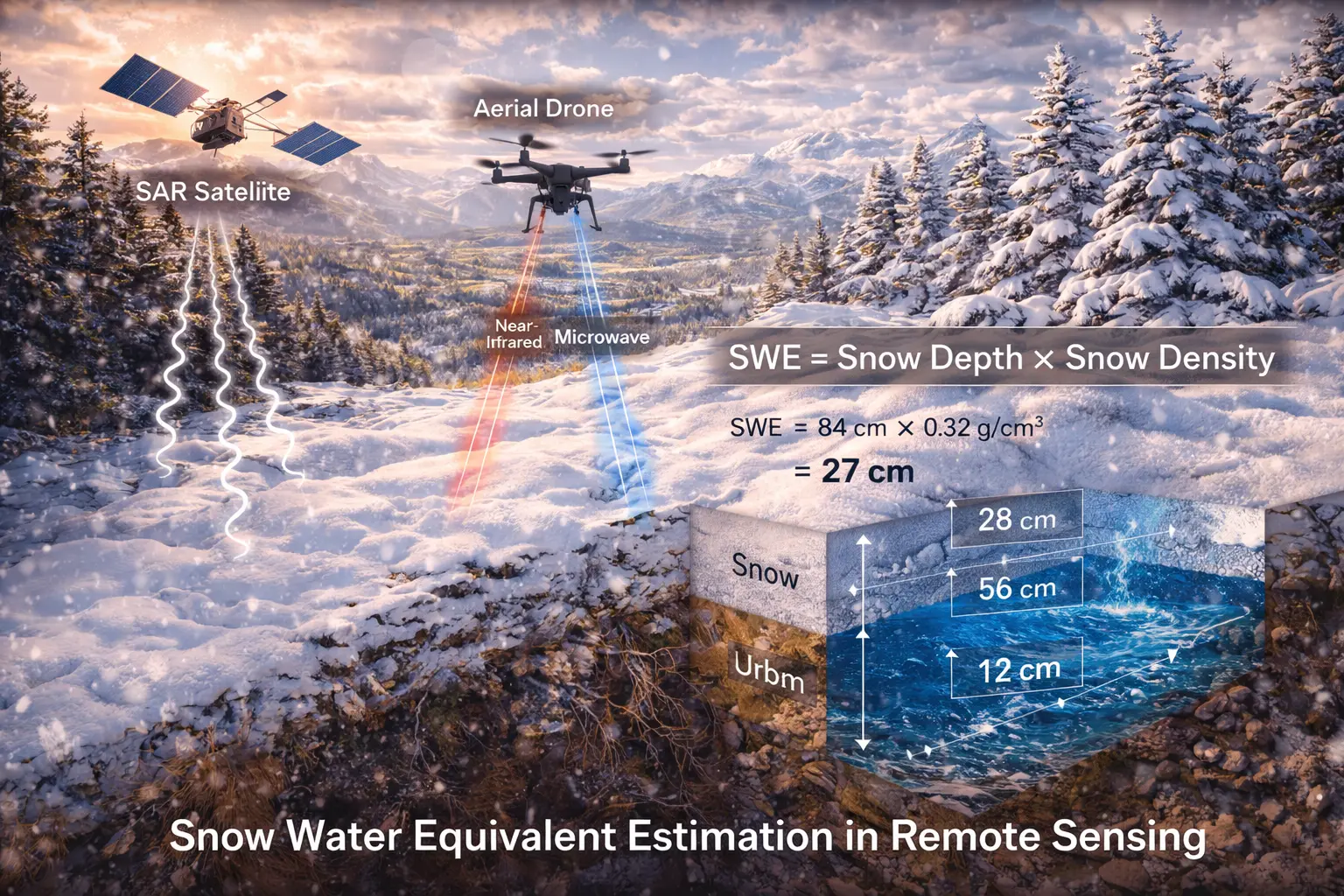
SWE From Snow Depth

Fundamental relationship:

\[\text{SWE} = \rho_{\text{snow}} \times d\]

Where:

$\rho_{\text{snow}}$ = bulk snow density (kg/m³)
$d$ = snow depth (m)

Challenge: Density varies (100-500 kg/m³) → must estimate.

Typical approach:

\[\rho_{\text{snow}} = \rho_0 + k_1 \text{DOY} + k_2 d\]

Where:

DOY = day of year (snow gets denser over time)
Coefficients calibrated regionally

Example (Colorado Rockies):

\[\rho = 250 + 0.5 \times \text{DOY} + 10 \times d\]

For March 15 (DOY 74), depth 1.5m:

\[\rho = 250 + 0.5(74) + 10(1.5) = 302 \text{ kg/m}^3\] \[\text{SWE} = 0.302 \times 1.5 = 0.453 \text{ m} = 453 \text{ mm}\]

Microwave Emission Theory

Snow emits microwave radiation based on:

Temperature
Depth
Grain size
Liquid water content

Brightness temperature:

\[T_B = T_{\text{snow}} \times (1 - e^{-\tau}) + T_{\text{ground}} \times e^{-\tau}\]

Where:

$T_B$ = brightness temperature measured by satellite (K)
$\tau$ = optical depth (function of SWE)
$T_{\text{snow}}$ = physical temperature of snow (K)
$T_{\text{ground}}$ = ground temperature (K)

Optical depth depends on SWE:

\[\tau = \beta \times \text{SWE}\]

Where $\beta$ = scattering coefficient (~0.002-0.005 m²/kg at 37 GHz).

Key insight: Deep snow → more scattering → lower $T_B$

Multi-Frequency Approach

Use two frequencies:

19 GHz (penetrates deep, insensitive to grain size)
37 GHz (scattered by snow grains)

Spectral gradient:

\[\Delta T_B = T_B(19\text{ GHz}) - T_B(37\text{ GHz})\]

Empirical SWE retrieval:

\[\text{SWE} = a \times \Delta T_B\]

Where $a \approx 3$ mm/K (calibration coefficient).

Positive $\Delta T_B$: Snow present (37 GHz scattered more)
Near zero: Little/no snow

3. Building the Mathematical Model

SNOTEL Snow Pillow

Measures weight of snowpack:

\[W = \rho_{\text{snow}} \times d \times A \times g\]

Where:

$W$ = weight (N)
$A$ = pillow area (m²)
$g$ = 9.81 m/s²

SWE directly:

\[\text{SWE} = \frac{W}{A \times \rho_w \times g}\]

Advantage: Direct measurement (no density assumption)

Disadvantage: Point measurement, expensive infrastructure

Manual Snow Course

Federal sampler:

Aluminum tube pushed through snowpack
Extract core
Weigh core

SWE calculation:

\[\text{SWE} = \frac{m_{\text{sample}}}{A_{\text{tube}} \times \rho_w}\]

Where:

$m_{\text{sample}}$ = mass of snow in tube (kg)
$A_{\text{tube}}$ = tube cross-section area (m²)

Typical: 10-12 sampling points along transect, average for site SWE.

Uncertainty: ±5-10% from sampling variability.

Passive Microwave Algorithm

Chang et al. (1987) algorithm:

For dry snow:

\[\text{SWE} = c_1 \times (T_B^{19V} - T_B^{37V}) \times f_{\text{forest}}\]

Where:

$c_1$ = 1.59 mm/K
$T_B^{19V}$ = 19 GHz vertical polarization (K)
$T_B^{37V}$ = 37 GHz vertical polarization (K)
$f_{\text{forest}}$ = forest correction factor

Forest correction:

\[f_{\text{forest}} = 1 - 0.8 \times f_c\]

Where $f_c$ = forest cover fraction (0-1).

Limitations:

Saturates at ~150mm SWE (deep snow)
Fails with wet snow (liquid water absorbs microwaves)
Coarse resolution (25 km pixels)

LiDAR Snow Depth

Airborne laser scanning:

Snow-on flight: Measure surface elevation $z_{\text{snow}}$

Snow-off flight: Measure bare ground elevation $z_{\text{ground}}$

Snow depth:

\[d = z_{\text{snow}} - z_{\text{ground}}\]

Convert to SWE:

\[\text{SWE} = \rho(x,y) \times d(x,y)\]

Density from:

Regional relationships
Interpolated from SNOTEL
modelled

Resolution: 1-3 meters (excellent for terrain effects)

Cost: Expensive (aircraft), limited temporal coverage

4. Worked Example by Hand

Problem: Estimate basin-average SWE from multiple sources.

Data:

SNOTEL stations (3 sites):

Low elevation (2000m): SWE = 300 mm
Mid elevation (2500m): SWE = 450 mm
High elevation (3000m): SWE = 600 mm

Passive microwave (basin average):

$\Delta T_B = 50$ K
SWE = $1.59 \times 50 = 79.5$ mm (underestimate due to saturation)

LiDAR (sample area, 2500m elevation):

Average depth: 1.8 m
Estimated density: 300 kg/m³
SWE = $0.300 \times 1.8 = 540$ mm

Basin characteristics:

Area: 500 km²
Elevation range: 1800-3200 m
Forest cover: 40%

Solution

Step 1: Elevation-based interpolation

Assume linear SWE-elevation relationship:

From SNOTEL:

2000m → 300mm
2500m → 450mm
3000m → 600mm

Gradient: $\frac{600 - 300}{3000 - 2000} = 0.30$ mm/m

SWE(z):

\[\text{SWE}(z) = 300 + 0.30(z - 2000)\]

Step 2: Basin hypsometry

Assume elevation distribution:

1800-2200m: 20% of area
2200-2600m: 40% of area
2600-3000m: 30% of area
3000-3200m: 10% of area

Average SWE per band:

Band 1 (2000m): SWE = 300mm → 20% × 300 = 60 mm
Band 2 (2400m): SWE = 420mm → 40% × 420 = 168 mm
Band 3 (2800m): SWE = 540mm → 30% × 540 = 162 mm
Band 4 (3100m): SWE = 630mm → 10% × 630 = 63 mm

Basin average: 60 + 168 + 162 + 63 = 453 mm

Step 3: Validate with LiDAR

LiDAR at 2500m: 540mm
Predicted at 2500m: 450mm

Difference: 90mm (20% higher)

Possible reasons:

Local accumulation pattern
Density uncertainty
Measurement error

Step 4: Final estimate

Best estimate: 453mm (from elevation interpolation)

Uncertainty: ±15% (±68mm)

Total water volume:

\[V = \text{SWE} \times A = 0.453 \text{ m} \times 500 \times 10^6 \text{ m}^2 = 226.5 \times 10^6 \text{ m}^3\]

= 226,500 acre-feet or 279 million cubic meters

5. Computational Implementation

Below is an interactive SWE estimation tool combining multiple sensors.

SNOTEL low (mm): 300 SNOTEL mid (mm): 450 SNOTEL high (mm): 600 Microwave ΔTB (K): 50

Basin avg SWE: -- mm

Total volume: -- million m³

Uncertainty: --%

Try this:

Red dots: SNOTEL station measurements
Blue line: Interpolated SWE-elevation relationship
Green bars: Elevation band SWE values
Orange dashed: Microwave satellite estimate (underestimates deep snow)
Adjust SNOTEL values: See gradient change
Microwave ΔTB: Higher = more snow detected (saturates ~150mm)
Notice: Microwave underestimates in deep snow (saturation issue)
Basin average combines elevation bands weighted by area

Key insight: Multiple sensors needed—ground stations for accuracy, satellites for coverage, models to bridge gaps!

6. Interpretation

SNOTEL Network

Automated stations:

Snow pillow (SWE)
Snow depth (ultrasonic)
Precipitation
Air temperature

US Western mountains: ~800 sites

Real-time data at https://www.nrcs.usda.gov/wps/portal/wcc/home/

Uses:

Water supply forecasting
Avalanche prediction
Climate monitoring
Model validation

NASA SnowEx Campaign

Multi-sensor airborne campaign:

Sensors:

Passive microwave radiometer
Active microwave (SAR, scatterometer)
LiDAR snow depth
Ground-penetrating radar (snow stratigraphy)

Goals:

Improve satellite algorithms
Understand uncertainty sources
Develop next-generation products

Findings:

Forest significantly attenuates microwave signal
Snow grain size affects scattering
Wet snow problematic for all microwave sensors

SWOT Satellite Mission

Surface Water and Ocean Topography (2022 launch):

Ka-band radar interferometry:

Measures water surface elevation
Rivers, lakes, reservoirs

Snow applications:

Seasonal water storage changes in reservoirs
Flood wave propagation
Groundwater-surface water exchange

Complements SWE observations for total water budget.

7. What Could Go Wrong?

Microwave Saturation

Deep snow (>150mm SWE):

Microwave signal saturates → underestimate.

Example:

True SWE: 800mm
Microwave estimate: 120mm
Error: -85%!

Worse in: Maritime climates (deep, wet snow)

Solution:

Combine with model
Use passive + active microwave
Assimilation techniques

Wet Snow

Liquid water absorbs microwaves.

Result: Brightness temperature increases (appears as less snow).

Example:

Dry snow: SWE = 300mm, ΔTB = 40K
After melt onset: Same SWE, ΔTB = 10K
Appears as: SWE decreased to 80mm (false!)

Solution: Freeze/thaw detection, temperature thresholding.

Forest Masking

Dense canopy:

Intercepts snow (different properties)
Emits radiation (masks snow signal)
Attenuates satellite view

Correction factors crude, uncertain.

Better: Higher frequency (e.g., 89 GHz) penetrates better, or use model.

Point-to-Grid Scaling

SNOTEL = point measurement (10m footprint)

Basin = 100s-1000s km²

Representativeness issues:

SNOTEL in clearings (higher SWE than forest)
Elevation bias (stations at accessible locations)
Aspect not captured

Solution: Distributed modelling with data assimilation.

8. Extension: Data Assimilation

Combine model with observations optimally.

Ensemble Kalman Filter (EnKF):

Steps:

Run snow model ensemble (100s of realizations with perturbed forcing)
Forecast SWE at observation time
Compare forecast to observations
Update ensemble using Kalman gain:

\[\mathbf{K} = \mathbf{P}^f \mathbf{H}^T (\mathbf{H}\mathbf{P}^f\mathbf{H}^T + \mathbf{R})^{-1}\]

Where:

$\mathbf{K}$ = Kalman gain
$\mathbf{P}^f$ = forecast error covariance
$\mathbf{H}$ = observation operator
$\mathbf{R}$ = observation error covariance

Analysis:

\[\mathbf{x}^a = \mathbf{x}^f + \mathbf{K}(\mathbf{y} - \mathbf{H}\mathbf{x}^f)\]

Result: Gridded SWE estimate that:

Respects physics (model)
Matches observations (data)
Quantifies uncertainty (ensemble spread)

Operational: NOAA National Water Model, NASA SWE reconstruction

9. Math Refresher: Electromagnetic Spectrum

Microwave Region

Frequency ranges:

Band	Frequency	Wavelength	Use
L	1-2 GHz	15-30 cm	Soil moisture
C	4-8 GHz	3.75-7.5 cm	Soil moisture, ice
X	8-12 GHz	2.5-3.75 cm	SAR imaging
Ku	12-18 GHz	1.67-2.5 cm	Precipitation
K	18-27 GHz	1.11-1.67 cm	Snow, water vapor
Ka	27-40 GHz	0.75-1.11 cm	Clouds, rain

Snow remote sensing: 19 GHz and 37 GHz most common

Why microwave?

Penetrates clouds (all-weather)
Sensitive to snow (grain scattering)
Day/night capable (active radiation)

Planck’s Law

Blackbody emission:

\[B_\nu(T) = \frac{2h\nu^3}{c^2} \frac{1}{e^{h\nu/kT} - 1}\]

Where:

$B_\nu$ = spectral radiance (W/(m²·sr·Hz))
$h$ = Planck constant
$\nu$ = frequency
$k$ = Boltzmann constant
$T$ = temperature (K)

Rayleigh-Jeans approximation (microwave regime):

\[B_\nu(T) \approx \frac{2\nu^2 kT}{c^2}\]

Brightness temperature: Temperature of blackbody that would produce observed radiance.

Summary

SWE estimation requires converting diverse measurements to water equivalent
Ground observations: SNOTEL (snow pillows), manual snow courses, direct SWE measurement
Passive microwave: Uses brightness temperature difference (19-37 GHz) to infer SWE
Microwave limitations: Saturates at ~150mm, fails with wet snow, forest attenuation
LiDAR: Accurate snow depth from airborne laser, requires density assumption
Scaling challenge: Point measurements to basin averages via elevation relationships
Multi-sensor fusion: Combines strengths of different platforms
Data assimilation: Optimal combination of models and observations (EnKF)
Operational products: SNOTEL network, AMSR-E/AMSR2, NASA SnowEx
Uncertainty: Typically ±15-25% for basin averages
Critical for water resources management and flood forecasting