Supervised Image Classification
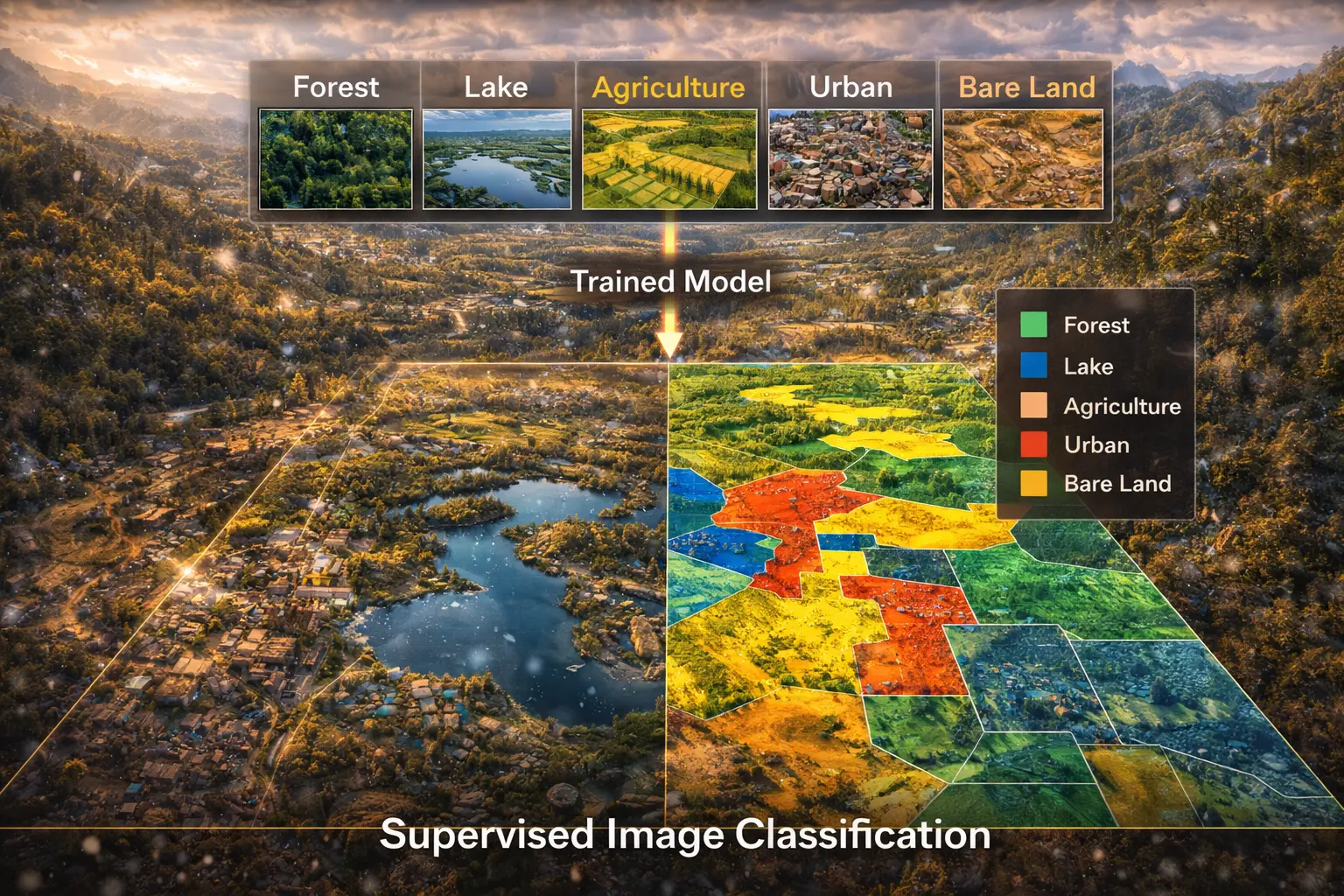
How do you convert satellite imagery to land cover maps? Supervised classification uses training samples to learn spectral signatures of each class, then classifies every pixel. This model derives maximum likelihood classification, implements k-nearest neighbors, and shows how to assess accuracy with confusion matrices.
Prerequisites: statistical classification, multivariate normal, maximum likelihood, feature space
1. The Question
How do you create a land cover map from a Landsat satellite image?
Image classification assigns every pixel to a category (class):
Land cover classes:
- Water
- Forest
- Urban/Built-up
- Agriculture (crops)
- Grassland/Pasture
- Barren land
Supervised classification workflow:
- Select training samples: Identify pixels of known class
- Extract signatures: Calculate spectral characteristics per class
- Train classifier: Learn decision boundaries in feature space
- Classify image: Assign every pixel to most likely class
- Assess accuracy: Compare results to ground truth
The mathematical question: Given training data (pixels with known labels) in multi-dimensional spectral space, how do we optimally classify unknown pixels?
2. The Conceptual Model
Feature Space
Each pixel is a point in n-dimensional space where n = number of bands.
Landsat 8 example (6 bands):
- Band 2 (Blue): 0.45-0.51 μm
- Band 3 (Green): 0.53-0.59 μm
- Band 4 (Red): 0.64-0.67 μm
- Band 5 (NIR): 0.85-0.88 μm
- Band 6 (SWIR1): 1.57-1.65 μm
- Band 7 (SWIR2): 2.11-2.29 μm
Pixel = 6D point: $(B_2, B_3, B_4, B_5, B_6, B_7)$
Classes form clusters in feature space:
- Water: Low NIR (absorbed), moderate visible
- Vegetation: Low red (chlorophyll absorption), high NIR (leaf scattering)
- Urban: Moderate across all bands
- Bare soil: Red-NIR similar, high SWIR
Training Data
Training samples: Pixels of known class (ground truth).
Collection methods:
- Field surveys (GPS + visual ID)
- High-resolution imagery interpretation
- Existing maps
- Expert knowledge
Requirements:
- Representative of class variability
- Spatially distributed across scene
- Sufficient quantity (50-100 pixels per class minimum)
Classification Algorithms
1. Maximum Likelihood (Parametric)
Assumes class signatures follow multivariate normal distribution.
Classifies to class with highest probability given pixel values.
2. K-Nearest Neighbors (Non-parametric)
Finds k closest training pixels in feature space.
Assigns majority class among neighbors.
3. Decision Trees / Random Forest
Learns hierarchical rules (if-then statements).
Ensembles of trees for robustness.
4. Support Vector Machines
Finds optimal hyperplanes separating classes.
Effective in high dimensions.
3. Building the Mathematical Model
Multivariate Normal Distribution
Class $i$ signature: Mean vector $\boldsymbol{\mu}_i$ and covariance matrix $\boldsymbol{\Sigma}_i$
For pixel with values $\mathbf{x} = (x_1, x_2, \ldots, x_n)$:
Probability density:
\[p(\mathbf{x} | C_i) = \frac{1}{(2\pi)^{n/2} |\boldsymbol{\Sigma}_i|^{1/2}} \exp\left(-\frac{1}{2}(\mathbf{x} - \boldsymbol{\mu}_i)^T \boldsymbol{\Sigma}_i^{-1} (\mathbf{x} - \boldsymbol{\mu}_i)\right)\]Where:
- $n$ = number of bands
-
$ \boldsymbol{\Sigma}_i $ = determinant of covariance matrix - $\boldsymbol{\Sigma}_i^{-1}$ = inverse of covariance matrix
Mahalanobis distance:
\[D_i^2 = (\mathbf{x} - \boldsymbol{\mu}_i)^T \boldsymbol{\Sigma}_i^{-1} (\mathbf{x} - \boldsymbol{\mu}_i)\]Measures distance in units of standard deviations (accounts for correlation).
Maximum Likelihood Classification
Bayes’ theorem:
\[P(C_i | \mathbf{x}) = \frac{p(\mathbf{x} | C_i) P(C_i)}{p(\mathbf{x})}\]Where:
-
$P(C_i \mathbf{x})$ = posterior probability (class given pixel) -
$p(\mathbf{x} C_i)$ = likelihood (pixel given class) - $P(C_i)$ = prior probability (class frequency)
- $p(\mathbf{x})$ = evidence (constant for all classes)
Classification rule:
\[\hat{C} = \arg\max_i P(C_i | \mathbf{x})\]Equivalent (taking log):
\[\hat{C} = \arg\max_i \left[\ln P(C_i) - \frac{1}{2}\ln|\boldsymbol{\Sigma}_i| - \frac{1}{2}D_i^2\right]\]If equal priors and equal covariances: Simplifies to minimum Mahalanobis distance.
K-Nearest Neighbors (k-NN)
Algorithm:
For pixel x:
    1. Calculate distance to all training pixels
    2. Find k nearest neighbors
    3. Count class frequencies among neighbors
    4. Assign majority class
Distance metric (Euclidean in feature space):
\[d(\mathbf{x}, \mathbf{x}_j) = \sqrt{\sum_{b=1}^{n} (x_b - x_{jb})^2}\]Typical k values: 3, 5, 7 (odd to avoid ties)
Pros: Simple, no distribution assumptions
Cons: Computationally expensive, sensitive to k choice
Accuracy Assessment
Confusion matrix: Cross-tabulation of predicted vs. actual classes.
Example:
| Water (pred) | Forest (pred) | Urban (pred) | |
|---|---|---|---|
| Water (true) | 85 | 2 | 3 |
| Forest (true) | 1 | 92 | 7 |
| Urban (true) | 5 | 6 | 89 |
Metrics:
Overall accuracy:
\[OA = \frac{\sum \text{diagonal}}{\text{total}} = \frac{85 + 92 + 89}{300} = 88.7\%\]Producer’s accuracy (recall):
\[PA_i = \frac{\text{correct}_i}{\text{reference total}_i}\]User’s accuracy (precision):
\[UA_i = \frac{\text{correct}_i}{\text{classified total}_i}\]Kappa coefficient: Agreement beyond chance
\[\kappa = \frac{OA - P_e}{1 - P_e}\]Where $P_e$ = expected accuracy by chance.
4. Worked Example by Hand
Problem: Classify a pixel using maximum likelihood.
Pixel values: Red = 0.10, NIR = 0.45
Training statistics (2 bands for simplicity):
Class 1 (Vegetation):
- Mean: $\boldsymbol{\mu}_1 = (0.08, 0.50)$ (low red, high NIR)
- Covariance: $\boldsymbol{\Sigma}_1 = \begin{pmatrix} 0.01 & 0 \ 0 & 0.02 \end{pmatrix}$
Class 2 (Soil):
- Mean: $\boldsymbol{\mu}_2 = (0.25, 0.30)$ (moderate both)
- Covariance: $\boldsymbol{\Sigma}_2 = \begin{pmatrix} 0.02 & 0 \ 0 & 0.02 \end{pmatrix}$
Assume equal priors: $P(C_1) = P(C_2) = 0.5$
Solution
Step 1: Compute Mahalanobis distance to each class
Class 1 (Vegetation):
\[\mathbf{x} - \boldsymbol{\mu}_1 = (0.10 - 0.08, 0.45 - 0.50) = (0.02, -0.05)\] \[\boldsymbol{\Sigma}_1^{-1} = \begin{pmatrix} 100 & 0 \\ 0 & 50 \end{pmatrix}\] \[D_1^2 = (0.02, -0.05) \begin{pmatrix} 100 & 0 \\ 0 & 50 \end{pmatrix} \begin{pmatrix} 0.02 \\ -0.05 \end{pmatrix}\] \[= (2, -2.5) \begin{pmatrix} 0.02 \\ -0.05 \end{pmatrix}\] \[= 0.04 + 0.125 = 0.165\]Class 2 (Soil):
\[\mathbf{x} - \boldsymbol{\mu}_2 = (0.10 - 0.25, 0.45 - 0.30) = (-0.15, 0.15)\] \[\boldsymbol{\Sigma}_2^{-1} = \begin{pmatrix} 50 & 0 \\ 0 & 50 \end{pmatrix}\] \[D_2^2 = (-0.15, 0.15) \begin{pmatrix} 50 & 0 \\ 0 & 50 \end{pmatrix} \begin{pmatrix} -0.15 \\ 0.15 \end{pmatrix}\] \[= (-7.5, 7.5) \begin{pmatrix} -0.15 \\ 0.15 \end{pmatrix}\] \[= 1.125 + 1.125 = 2.25\]Step 2: Compute discriminant function
| Assume equal covariances → ignore $\ln | \boldsymbol{\Sigma}_i | $ term |
Class 1: $g_1 = \ln(0.5) - 0.5(0.165) = -0.693 - 0.083 = -0.776$
Class 2: $g_2 = \ln(0.5) - 0.5(2.25) = -0.693 - 1.125 = -1.818$
Step 3: Classify
\[\max(g_1, g_2) = \max(-0.776, -1.818) = -0.776\]Classification: Vegetation (Class 1)
Interpretation: Pixel is closer to vegetation signature (low red, high NIR).
5. Computational Implementation
Below is an interactive image classification demo.
Classes: Water (blue), Vegetation (green), Urban (gray), Bare soil (brown)
Overall accuracy: --%
Try this:
- Maximum likelihood: Statistical classification based on class distributions
- K-nearest neighbors: Non-parametric, uses nearest training samples
- Minimum distance: Simplest method, distance to class means
- Feature space plot: Shows class separation in Red-NIR space
- Training samples: White boxes show training regions
- Color legend: Blue (water), Green (vegetation), Gray (urban), Brown (soil)
- Notice: Classes cluster in feature space—high NIR separates vegetation!
Key insight: Spectral signatures enable automatic land cover mapping from satellite imagery!
6. Interpretation
Global Land Cover Mapping
Products:
- MODIS Land Cover (500m, annual, 2001-present)
- ESA CCI Land Cover (300m, annual, 1992-2020)
- FROM-GLC (30m, Landsat-based)
Uses:
- Climate modelling (surface albedo, roughness)
- Carbon cycle (vegetation biomass)
- Agriculture monitoring
- Urban growth tracking
Crop Type Mapping
USDA Cropland Data Layer (30m, annual, US):
- Corn vs. soybeans vs. wheat
- Training: Field surveys + farmer reports
- Accuracy: >90% for major crops
Applications:
- Yield prediction
- Irrigation demand
- Crop insurance
- Policy planning
Forest Mapping
Forest/non-forest:
- Binary classification (easier, higher accuracy)
- Global Forest Change product (Hansen et al.)
- 30m resolution, 2000-2023
Forest type:
- Deciduous vs. evergreen vs. mixed
- Requires phenology (time series)
7. What Could Go Wrong?
Insufficient Training Data
Small sample size → Poor class statistics → Misclassification
Solution:
- Collect 50-100 pixels per class minimum
- Ensure spatial distribution across scene
- Include class variability (e.g., young vs. mature forest)
Class Confusion
Spectrally similar classes:
- Dry grass vs. bare soil
- Urban vs. bare rock
- Shallow water vs. wet sand
Separability analysis:
\[D_{ij} = \frac{||\boldsymbol{\mu}_i - \boldsymbol{\mu}_j||^2}{\sigma_i^2 + \sigma_j^2}\]Low separability (< 1.0): Consider merging classes or adding bands.
Shadow and Topography
Terrain shadows reduce brightness → misclassified as water.
Solution:
- Topographic correction (normalize for solar angle + slope)
- Use indices less sensitive to illumination (e.g., NDVI)
Mixed Pixels
30m Landsat pixel may contain multiple cover types:
- Edge between forest and field
- Urban with scattered vegetation
Sub-pixel classification:
- Estimate fractional cover (30% forest, 70% grass)
- Spectral unmixing algorithms
8. Extension: Random Forest Classification
Ensemble of decision trees.
Algorithm:
For each tree:
    1. Bootstrap sample of training data
    2. At each node:
       - Select random subset of features
       - Find best split on these features
    3. Grow tree to maximum depth
    4. Store tree

Classification:
    - Each tree votes
    - Assign majority class
Advantages:
- Handles non-linear relationships
- Robust to outliers
- Feature importance ranking
- High accuracy
Disadvantages:
- Black box (hard to interpret)
- Computationally intensive
Widely used in operational land cover mapping.
9. Math Refresher: Multivariate Normal Distribution
Univariate Normal
1D Gaussian:
\[p(x | \mu, \sigma^2) = \frac{1}{\sqrt{2\pi\sigma^2}} \exp\left(-\frac{(x-\mu)^2}{2\sigma^2}\right)\]Parameters: Mean $\mu$, variance $\sigma^2$
68-95-99.7 rule: 68% within 1σ, 95% within 2σ, 99.7% within 3σ
Multivariate Normal
n-dimensional:
\[p(\mathbf{x} | \boldsymbol{\mu}, \boldsymbol{\Sigma}) = \frac{1}{(2\pi)^{n/2}|\boldsymbol{\Sigma}|^{1/2}} \exp\left(-\frac{1}{2}(\mathbf{x}-\boldsymbol{\mu})^T\boldsymbol{\Sigma}^{-1}(\mathbf{x}-\boldsymbol{\mu})\right)\]Parameters:
- Mean vector $\boldsymbol{\mu} = (\mu_1, \mu_2, \ldots, \mu_n)$
- Covariance matrix $\boldsymbol{\Sigma}$ (n×n, symmetric, positive definite)
Covariance:
\[\Sigma_{ij} = \text{Cov}(X_i, X_j) = E[(X_i - \mu_i)(X_j - \mu_j)]\]Diagonal elements: Variances $\sigma_i^2$
Off-diagonal: Covariances (measure linear relationship)
Mahalanobis distance:
\[D^2 = (\mathbf{x}-\boldsymbol{\mu})^T\boldsymbol{\Sigma}^{-1}(\mathbf{x}-\boldsymbol{\mu})\]Generalizes Euclidean distance, accounting for variance and correlation.
Summary
- Supervised classification uses training samples to learn class signatures
- Feature space: Each pixel is a point in n-dimensional spectral space
- Maximum likelihood: Assumes multivariate normal, classifies to highest probability
- K-nearest neighbors: Non-parametric, assigns majority class among k nearest training pixels
- Mahalanobis distance: Accounts for variance and correlation in feature space
- Accuracy assessment: Confusion matrix, overall accuracy, producer’s/user’s accuracy, kappa
- Applications: Global land cover, crop mapping, forest monitoring
- Challenges: Class confusion, shadows, mixed pixels, insufficient training
- Random forest: Ensemble method with high accuracy for complex classifications
- Foundation of operational remote sensing land cover products