Raster Classification and Reclassification
Convert elevation to slope classes. Transform NDVI to vegetation categories. Turn temperature into climate zones. Classification transforms continuous raster values into discrete categories using thresholds, ranges, and decision rules. This model derives classification methods and shows how to choose breakpoints.
Prerequisites: thresholding, decision rules, classification schemes, histogram analysis
1. The Question
How do you convert a continuous elevation raster into slope classes: “flat”, “gentle”, “steep”, “very steep”?
Reclassification transforms raster values using decision rules:
Examples:
- Slope categories: 0-5° = flat, 5-15° = gentle, 15-30° = steep, >30° = very steep
- Land cover from NDVI: <0.2 = bare, 0.2-0.4 = sparse veg, 0.4-0.6 = moderate, >0.6 = dense
- Habitat suitability: Combine elevation + slope + aspect into “suitable” vs “unsuitable”
- Fire risk zones: Temperature + humidity + vegetation → low/medium/high risk
The mathematical question: Given continuous input values, how do we assign them to discrete classes efficiently and meaningfully?
Key decisions:
- Number of classes: Too few → information loss; too many → complexity
- Breakpoints: Where to split? Equal intervals? Natural breaks? Quantiles?
- Edge handling: Is 15.0° “gentle” or “steep”?
2. The Conceptual Model
Classification vs. Reclassification
Classification: Assign raw values to meaningful categories
- Satellite imagery → land cover classes
- Temperature values → climate zones
Reclassification: Transform one categorical raster to another
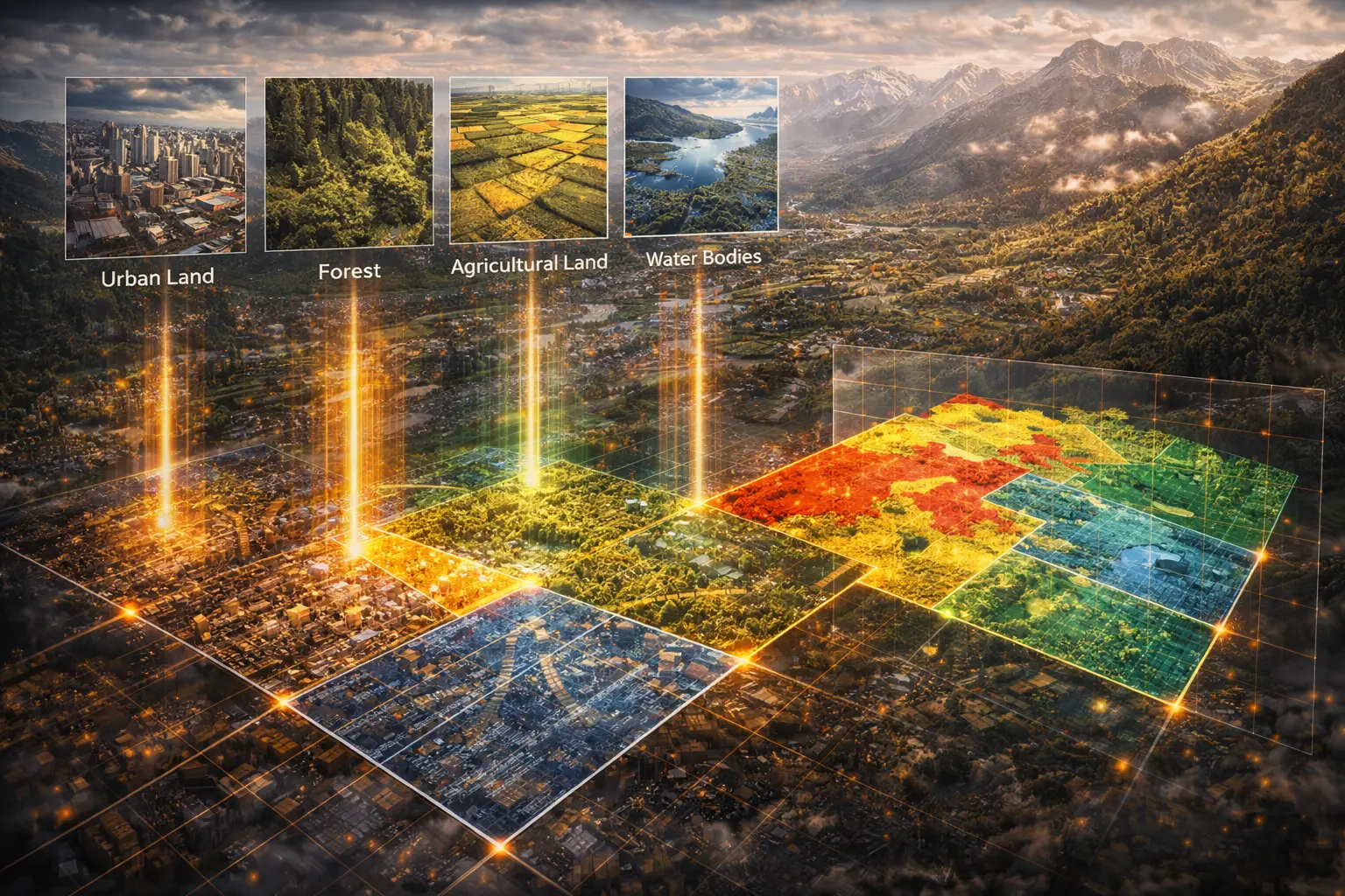
- 10 land cover types → 3 broad categories (urban/forest/agriculture)
- Detailed soil types → simplified drainage classes
Both use the same mathematical framework.
Classification Schemes
1. Equal Interval
Divide value range into equal-width bins.
\[\text{Class } i: \left[\min + i \cdot \frac{\max - \min}{n}, \min + (i+1) \cdot \frac{\max - \min}{n}\right)\]Example: Elevation 0-1000m, 5 classes → each class spans 200m
Pros: Simple, intuitive
Cons: May have empty classes or very unbalanced distribution
2. Quantiles (Equal Count)
Each class contains equal number of pixels.
k% quantile: Value below which k% of data falls.
Example: 4 classes → breakpoints at 25th, 50th, 75th percentiles
Pros: Balanced class sizes
Cons: Breakpoints may not align with natural boundaries
3. Natural Breaks (Jenks)
Minimize within-class variance, maximize between-class variance.
Objective: Find breaks that create most homogeneous classes.
Algorithm: Dynamic programming to optimize:
\[\min \sum_{i=1}^{k} \sum_{x \in \text{class}_i} (x - \bar{x}_i)^2\]Pros: Respects data distribution
Cons: Computationally expensive, breakpoints change with data
4. Standard Deviation
Classes based on deviations from mean.
\[\text{Class boundaries: } \mu - 2\sigma, \mu - \sigma, \mu, \mu + \sigma, \mu + 2\sigma\]Pros: Statistical meaning (normal distribution)
Cons: Assumes normal distribution (often violated)
5. Manual/Expert
Domain expert specifies meaningful thresholds.
Example: Slope classes from geomorphology literature
- 0-2°: Flat (flooding possible)
- 2-5°: Gentle (easy to build on)
- 5-15°: Moderate (erosion risk increases)
- 15-30°: Steep (difficult access)
-
30°: Very steep (landslide risk)
Pros: Incorporates domain knowledge
Cons: Subjective, may not fit specific dataset
3. Building the Mathematical Model
Simple Threshold Classification
Binary classification:
\[z_{\text{out}} = \begin{cases} 1 & \text{if } z_{\text{in}} \geq T \\ 0 & \text{if } z_{\text{in}} < T \end{cases}\]Example: Water detection from elevation
- Threshold $T = 0$ m (sea level)
- Output: 1 = land, 0 = water
Multi-Class Range Classification
Define breakpoints: $b_0 < b_1 < b_2 < \cdots < b_n$
Classification function:
\[\text{class}(z) = \begin{cases} 1 & \text{if } b_0 \leq z < b_1 \\ 2 & \text{if } b_1 \leq z < b_2 \\ \vdots \\ n & \text{if } b_{n-1} \leq z < b_n \end{cases}\]Implementation:
def classify(value, breaks):
    for i, break_value in enumerate(breaks[1:]):
        if value < break_value:
            return i + 1
    return len(breaks)
Lookup Table Reclassification
Map specific input values to output values.
Lookup table:
| Input Value | Output Value |
|---|---|
| 1 (Forest) | 1 (Vegetation) |
| 2 (Grass) | 1 (Vegetation) |
| 3 (Crops) | 1 (Vegetation) |
| 4 (Urban) | 2 (Developed) |
| 5 (Water) | 3 (Water) |
Function:
\[z_{\text{out}} = \text{LUT}[z_{\text{in}}]\]Efficient with arrays/dictionaries.
Fuzzy Classification
Instead of hard boundaries, use membership functions.
Example - “Moderate slope” membership:
\[\mu_{\text{moderate}}(s) = \begin{cases} 0 & s < 5 \\ \frac{s - 5}{10} & 5 \leq s < 15 \\ 1 & 15 \leq s < 25 \\ \frac{35 - s}{10} & 25 \leq s < 35 \\ 0 & s \geq 35 \end{cases}\]Value between 0 and 1 indicates degree of membership.
Advantage: Represents uncertainty at boundaries.
4. Worked Example by Hand
Problem: Classify this temperature raster (°C) into 3 categories using equal intervals.
Input:
    j=0  j=1  j=2  j=3
i=0  10   15   20   25
i=1  12   18   22   28
i=2  14   16   24   30
i=3  11   19   26   32
Categories:
- Cold (1)
- Moderate (2)
- Hot (3)
Solution
Step 1: Find range
\(\min = 10°C, \quad \max = 32°C\) \(\text{range} = 32 - 10 = 22°C\)
Step 2: Calculate interval width
\[\text{width} = \frac{22}{3} = 7.33°C\]Step 3: Define breakpoints
- $b_0 = 10$
- $b_1 = 10 + 7.33 = 17.33$
- $b_2 = 17.33 + 7.33 = 24.67$
- $b_3 = 32$
Classes:
- Cold (1): [10, 17.33)
- Moderate (2): [17.33, 24.67)
- Hot (3): [24.67, 32]
Step 4: Classify each cell
Row 0:
- 10 < 17.33 → 1 (Cold)
- 15 < 17.33 → 1
- 20 ∈ [17.33, 24.67) → 2 (Moderate)
- 25 ≥ 24.67 → 3 (Hot)
Row 1:
- 12 → 1, 18 → 2, 22 → 2, 28 → 3
Row 2:
- 14 → 1, 16 → 1, 24 → 2, 30 → 3
Row 3:
- 11 → 1, 19 → 2, 26 → 3, 32 → 3
Output:
    j=0  j=1  j=2  j=3
i=0   1    1    2    3
i=1   1    2    2    3
i=2   1    1    2    3
i=3   1    2    3    3
Class counts:
- Cold (1): 6 cells
- Moderate (2): 6 cells
- Hot (3): 4 cells
Not perfectly balanced (would be 5.33 each) because we used equal intervals, not quantiles.
5. Computational Implementation
Below is an interactive raster classification tool.
Try this:
- Equal interval: Fixed-width bins (may be unbalanced)
- Quantile: Balanced class sizes (breaks at data percentiles)
- Standard deviation: Statistical bins (assumes normal distribution)
- Manual: Set your own thresholds (red lines on histogram)
- Adjust class count: See how distribution changes
- Histogram: Red lines show where breaks occur in data
Key insight: Method choice dramatically affects results—no single “correct” classification.
6. Interpretation
Slope Classification Example
From DEM to actionable information:
1. Calculate slope (degrees) from DEM
2. Classify:
   - 0-2°: Suitable for farming, flooding risk
   - 2-5°: Good for construction
   - 5-15°: Moderate difficulty, erosion control needed
   - 15-30°: Forestry, recreation only
   - >30°: Hazard zones, protect from development
Result: Planning tool, not just numbers.
NDVI to Land Cover
Thresholds from literature:
NDVI < 0.1: Water, barren land
0.1-0.2: Sparse vegetation (desert)
0.2-0.4: Grassland, shrubland
0.4-0.6: Cropland, mixed vegetation
0.6-0.8: Dense vegetation (forest)
>0.8: Very dense vegetation (rainforest)
Validated against ground truth from field surveys.
Multi-Criteria Suitability
Combine multiple factors:
slope_class = classify(slope, [0, 5, 15, 30])
aspect_class = classify(aspect, [0, 90, 180, 270, 360])
soil_class = reclassify(soil_type, lookup_table)

suitability = (slope_class == 1) AND
              (aspect_class IN [2, 3]) AND
              (soil_class IN [1, 2])
Boolean result: Suitable (1) or not (0).
7. What Could Go Wrong?
Arbitrary Breakpoints
Equal interval on skewed data:
Data: [1, 1, 2, 2, 2, 3, 3, 50]
Equal intervals (4 classes):
  [1, 13.25): 7 values → Class 1
  [13.25, 25.5): 0 values → Class 2
  [25.5, 37.75): 0 values → Class 3
  [37.75, 50]: 1 value → Class 4
Problem: Empty classes, unbalanced.
Solution: Use quantiles or remove outliers first.
Sensitivity to Outliers
One extreme value shifts all breakpoints:
Data: [10, 12, 14, 15, 16, 18, 20, 1000]
Equal intervals with outlier → huge bins
Solution:
- Remove outliers before classification
- Use robust statistics (median, IQR)
- Clip extreme values
Loss of Information
Continuous to categorical loses detail:
Original: 15.2°, 15.8° (0.6° difference)
Classified: Both → Class 2 "gentle" (appear identical)

Original: 14.9°, 15.1° (0.2° difference)
Classified: 14.9° → Class 1, 15.1° → Class 2 (appear very different)
Problem: Boundary artifacts.
Solution: Use buffer zones or fuzzy classification.
Inappropriate Method
Quantiles on categorical data:
Land cover codes: [1, 1, 1, 2, 2, 3, 3, 3]
Quantile classification → meaningless
Solution: Only classify continuous data. Reclassify categorical via lookup tables.
8. Extension: Unsupervised Classification
Automated clustering finds natural groups in data.
K-means algorithm:
1. Initialize k cluster centers randomly
2. Assign each pixel to nearest center
3. Recompute centers as mean of assigned pixels
4. Repeat 2-3 until convergence
For multi-band imagery:
pixel = [band1, band2, band3, ..., bandN]
distance = sqrt(sum((pixel - center)²))
Advantage: No manual thresholds needed.
Disadvantage: Classes may not align with semantic categories.
Example: Classify Landsat image (7 bands) into 10 land cover types automatically.
9. Math Refresher: Quantiles and Percentiles
Definition
p-th quantile ($Q_p$): Value below which fraction $p$ of data falls.
Example: Median = 0.5 quantile (50th percentile)
Calculation
For sorted data $x_1 \leq x_2 \leq \cdots \leq x_n$:
Position:
\[\text{pos} = p \times (n - 1) + 1\]If position is integer: $Q_p = x_{\text{pos}}$
If fractional: Interpolate between $x_{\lfloor\text{pos}\rfloor}$ and $x_{\lceil\text{pos}\rceil}$
Example: Find 0.25 quantile of [1, 2, 3, 4, 5]
\[\text{pos} = 0.25 \times (5 - 1) + 1 = 2\] \[Q_{0.25} = x_2 = 2\]For Classification
Divide into k equal-count classes:
Breakpoints at quantiles: $Q_{1/k}, Q_{2/k}, \ldots, Q_{(k-1)/k}$
Example: 4 classes → breaks at 0.25, 0.5, 0.75 quantiles
Summary
- Classification converts continuous rasters to discrete categories
- Five methods: Equal interval, quantile, natural breaks, standard deviation, manual
- Equal interval: Fixed-width bins, simple but may be unbalanced
- Quantile: Equal-count bins, balanced but may group dissimilar values
- Natural breaks: Minimizes within-class variance, computationally expensive
- Manual thresholds: Domain expert knowledge, most meaningful for applications
- Reclassification: Uses lookup tables to transform categorical rasters
- Fuzzy classification: Membership functions instead of hard boundaries
- Applications: Slope classes, land cover mapping, suitability analysis
- Challenges: Outliers, information loss, boundary artifacts
- Method choice depends on data distribution and application requirements
This completes Cluster K (Raster Foundations)! We’ve covered resampling (33), map algebra (34), and classification (35).
Next: Model 36 launches Cluster M (Terrain Analysis) with viewshed and line-of-sight analysis!