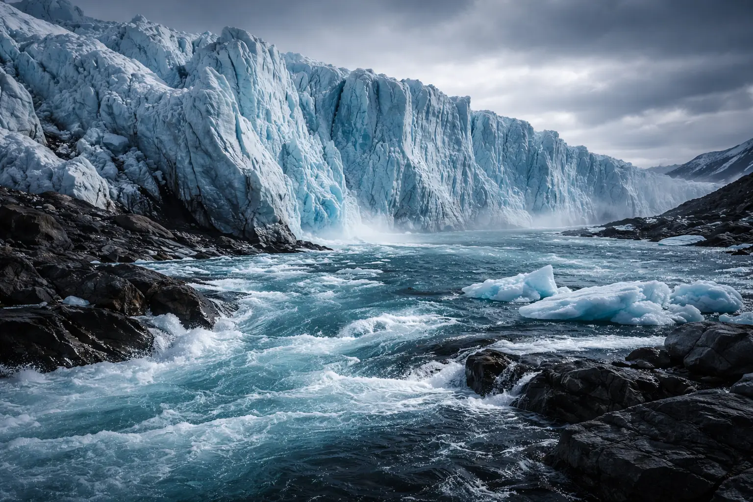
Glacial Meltwater Chemistry
Why is glacial meltwater so turbid and mineralized? Glaciers grind bedrock to fine powder, creating massive rock-water contact. Meltwater chemistry reveals residence time, weathering reactions, and mixing sources. This model derives weathering rates, implements mixing models, and shows how glacial chemistry affects downstream ecosystems and water resources.
Prerequisites: chemical weathering, solute transport, mixing models, ionic balance
1. The Question
Why does glacial meltwater look milky and taste mineral-rich?
Glacial meltwater characteristics:
Physical:
- High turbidity (suspended sediment)
- Cold temperature (0-4°C)
- Variable discharge (diurnal, seasonal)
- Milky appearance (“glacial flour”)
Chemical:
- High total dissolved solids (TDS)
- Elevated Ca²⁺, Mg²⁺, SO₄²⁻
- Low organic carbon
- Neutral to slightly alkaline pH (7-8.5)
- High weathering rates
Why different from rainwater?
Long rock-water contact + fresh mineral surfaces + mechanical grinding = rapid chemical weathering
2. The Conceptual Model
Weathering Reactions
1. Carbonate dissolution (fast):
\[\text{CaCO}_3 + \text{CO}_2 + \text{H}_2\text{O} \rightarrow \text{Ca}^{2+} + 2\text{HCO}_3^-\]Products: Calcium, bicarbonate
Rate: Hours to days
Result: Dominates early meltwater
2. Silicate hydrolysis (slow):
$$2\text{NaAlSi}_3\text{O}_8 + 2\text{CO}_2 + 11\text{H}_2\text{O} \rightarrow \text{Al}_2\text{Si}_2\text{O}_5(\text{OH})_4 + 2\text{Na}^+ + 2\text{HCO}_3^- + 4\text{H}_4\text{SiO}_4$$
(Albite → Kaolinite)
Products: Sodium, bicarbonate, silica
Rate: Months to years
Result: Subglacial residence increases silicate contribution
3. Sulfide oxidation:
$$2\text{FeS}_2 + 7\text{O}_2 + 2\text{H}_2\text{O} \rightarrow 2\text{Fe}^{2+} + 4\text{SO}_4^{2-} + 4\text{H}^+$$
Products: Iron, sulfate, acidity
Rate: Variable
Result: Low pH in some glacial streams
Three Water Sources
Supraglacial (surface):
- Snowmelt, ice melt
- Short residence time (hours)
- Low solute concentration
- Low turbidity
Englacial (within ice):
- Melt from crevasses, moulins
- Moderate residence time (days)
- Moderate solute concentration
- Moderate turbidity
Subglacial (beneath ice):
- Melt at glacier bed
- Long residence time (weeks-months)
- High solute concentration
- Very high turbidity (crushing bedrock)
Mixing:
\[C_{\text{stream}} = f_{\text{supra}} C_{\text{supra}} + f_{\text{en}} C_{\text{en}} + f_{\text{sub}} C_{\text{sub}}\]Where $f_i$ = fraction from each source, $\sum f_i = 1$
Diurnal Cycle
Daytime (peak melt):
- High discharge
- More supraglacial contribution
- Lower solute concentration (dilution)
- Higher turbidity (sediment flushing)
Nighttime (low melt):
- Low discharge
- More subglacial contribution
- Higher solute concentration
- Lower turbidity (settling)
Hysteresis: Concentration vs. discharge traces loop (not 1:1 relationship)
3. Building the Mathematical Model
Chemical Denudation Rate
Mass of dissolved material per unit area per time:
\[D_{\text{chem}} = \frac{Q \times C}{A}\]Where:
- $D_{\text{chem}}$ = chemical denudation rate (kg/m²/year or mm/year bedrock equivalent)
- $Q$ = runoff (m³/year)
- $C$ = solute concentration (kg/m³ = g/L)
- $A$ = catchment area (m²)
Convert to bedrock-equivalent erosion rate:
\[E_{\text{chem}} = \frac{D_{\text{chem}}}{\rho_{\text{rock}}}\]Where $\rho_{\text{rock}} \approx 2700$ kg/m³
Typical glacial catchments:
- $D_{\text{chem}} = 50-200$ kg/m²/year
- $E_{\text{chem}} = 0.02-0.08$ mm/year
Compare to mechanical erosion: 0.5-5 mm/year (glaciers erode 10-100× faster mechanically than chemically)
Weathering Rate Constant
First-order kinetics:
\[\frac{dC}{dt} = k (C_{\text{eq}} - C)\]Where:
- $k$ = rate constant (s⁻¹)
- $C_{\text{eq}}$ = equilibrium concentration
- $C$ = current concentration
Solution (with residence time $\tau$):
\[C(\tau) = C_{\text{eq}} (1 - e^{-k\tau})\]Short residence: $C \ll C_{\text{eq}}$ (kinetically limited)
Long residence: $C \rightarrow C_{\text{eq}}$ (equilibrium)
Typical subglacial: $k \sim 10^{-6}$ to $10^{-5}$ s⁻¹
Two-Component Mixing Model
Solve for subglacial fraction:
Given:
- $C_{\text{stream}}$ = measured concentration
- $C_{\text{supra}}$ = supraglacial endmember
- $C_{\text{sub}}$ = subglacial endmember
Simple two-source:
\[f_{\text{sub}} = \frac{C_{\text{stream}} - C_{\text{supra}}}{C_{\text{sub}} - C_{\text{supra}}}\] \[f_{\text{supra}} = 1 - f_{\text{sub}}\]Multi-tracer approach uses multiple solutes simultaneously (Ca²⁺, SO₄²⁻, δ¹⁸O) to constrain mixing better.
Suspended Sediment Concentration
Empirical relationship with discharge:
\[\text{SSC} = a Q^b\]Where:
- SSC = suspended sediment concentration (mg/L)
- $Q$ = discharge (m³/s)
- $a, b$ = empirical constants
Glacial streams: $b \approx 0.5-0.8$ (positive relationship but sub-linear)
Why sub-linear? Sediment supply limited at high flows (source exhaustion).
4. Worked Example by Hand
Problem: Calculate chemical denudation rate and mixing.
Data:
Catchment:
- Area: 10 km²
- Annual runoff: 2000 mm/year
Stream chemistry (annual mean):
- Ca²⁺: 45 mg/L
- Mg²⁺: 15 mg/L
- Na⁺: 10 mg/L
- SO₄²⁻: 80 mg/L
- HCO₃⁻: 150 mg/L
- Total Dissolved Solids (TDS): 300 mg/L
Endmembers:
- Supraglacial: TDS = 10 mg/L
- Subglacial: TDS = 800 mg/L
Solution
Step 1: Chemical denudation
Annual runoff volume:
\[Q = 2000 \text{ mm/year} \times 10 \times 10^6 \text{ m}^2 = 2 \times 10^{10} \text{ L/year}\]Mass of dissolved material:
\[M = C \times Q = 300 \text{ mg/L} \times 2 \times 10^{10} \text{ L/year} = 6 \times 10^{12} \text{ mg/year} = 6 \times 10^6 \text{ kg/year}\]Denudation rate:
\[D_{\text{chem}} = \frac{6 \times 10^6}{10 \times 10^6} = 0.6 \text{ kg/m}^2\text{/year}\]Step 2: Bedrock-equivalent erosion
\[E_{\text{chem}} = \frac{0.6}{2700} = 0.00022 \text{ m/year} = 0.22 \text{ mm/year}\]Step 3: Mixing calculation
\[f_{\text{sub}} = \frac{300 - 10}{800 - 10} = \frac{290}{790} = 0.37 = 37\%\] \[f_{\text{supra}} = 1 - 0.37 = 0.63 = 63\%\]Interpretation:
- Annual average: 63% supraglacial, 37% subglacial
- Chemical denudation: 0.6 kg/m²/year (moderate)
- Bedrock erosion equivalent: 0.22 mm/year (slow compared to mechanical)
Variation: Summer likely >80% supraglacial (high melt), winter <20% supraglacial (baseflow from subglacial storage)
5. Computational Implementation
Below is an interactive glacial chemistry simulator.
Discharge: -- m³/s
TDS: -- mg/L
Subglacial %: --%
SSC: -- mg/L
Try this:
- Slide through day: See discharge peak at noon (blue), TDS minimum (green)
- Summer vs Fall: Higher discharge in summer, more dilution
- Carbonate bedrock: Very high TDS (limestone dissolves rapidly)
- Silicate bedrock: Lower TDS (granite dissolves slowly)
- Blue area: Discharge (peaks afternoon)
- Green line: Total dissolved solids (inverse relationship!)
- Orange dashed: Subglacial contribution % (higher at night)
- Red vertical: Current time marker
- Notice: High flow = low concentration (dilution), low flow = high concentration (subglacial dominates)!
Key insight: Chemistry and discharge show hysteresis—the loop reveals mixing processes and water sources!
6. Interpretation
Glacier Contribution to Ocean Chemistry
Global glacial runoff: ~3000 km³/year
Chemical flux to oceans:
- Ca²⁺: ~50 × 10⁹ mol/year
- HCO₃⁻: ~100 × 10⁹ mol/year
- Silica: ~10 × 10⁹ mol/year
CO₂ drawdown:
Silicate weathering consumes atmospheric CO₂:
\[\text{CO}_2 + \text{CaSiO}_3 \rightarrow \text{CaCO}_3 + \text{SiO}_2\]Glacial contribution: ~1-2% of global silicate weathering (though glaciers cover <1% land area → high rates per area!)
Ecosystem Effects
Downstream impacts:
Positive:
- Nutrient delivery (Fe, P from rock flour)
- Supports phytoplankton blooms in fjords
- Cold water refugia for salmon
Negative:
- High turbidity limits light (reduces primary production)
- Temperature stress (too cold for some species)
- Variable flow regime (habitat instability)
Example - Gulf of Alaska:
- Glacial sediment plumes visible from space
- Fe delivery supports productive fisheries
- Climate change → changing timing and magnitude
Water Resources
Drinking water:
- Low organic content (good)
- High turbidity (expensive filtration)
- Variable mineralization (treatment complexity)
Hydropower:
- Sediment abrasion of turbines (costly)
- Variable flow (generation uncertainty)
Agriculture:
- Reliable summer irrigation
- But declining as glaciers shrink
7. What Could Go Wrong?
Assuming Steady Endmembers
Reality: Endmember composition varies:
Subglacial TDS varies with:
- Season (winter storage → more concentrated)
- Flow path evolution (channelized vs distributed)
- Bedrock heterogeneity
Solution: Collect endmember samples throughout season, use ranges.
Ignoring Precipitation Chemistry
Rain/snow has solutes too:
- Sea salt aerosols (coastal)
- Dust deposition
- Anthropogenic inputs (acid rain)
Can be 10-30% of stream chemistry in some cases.
Solution: Include precipitation endmember in mixing model.
Sample Timing
Grab samples miss variability:
Daily: Diurnal cycle (factor of 2-3× concentration range)
Seasonal: Summer vs winter (order of magnitude difference)
Solution:
- Flow-weighted composite sampling
- Automated samplers
- High-frequency sensors (conductivity as TDS proxy)
Suspended vs Dissolved
Glacial flour (suspended):
- Not dissolved, but measured in “total” analyses
- Settles out in reservoirs
Dissolved load:
- Truly in solution
- Remains through settling
Must distinguish for chemical denudation calculations.
8. Extension: Isotope Tracers
Stable isotopes reveal water sources and processes:
δ¹⁸O and δD (deuterium):
Snowmelt: Depleted (negative values)
Ice melt: Very depleted (ancient precipitation)
Rain: Enriched (positive values)
Mixing equation:
\[\delta_{\text{stream}} = f_{\text{snow}} \delta_{\text{snow}} + f_{\text{ice}} \delta_{\text{ice}} + f_{\text{rain}} \delta_{\text{rain}}\]Combined with chemistry:
3 endmembers × 3 tracers (δ¹⁸O, TDS, SO₄²⁻) → solve for fractions
Tritium (³H):
Bomb peak (1960s): High values
Old ice: Pre-bomb, very low
Dates water (ice age determination)
9. Math Refresher: Mass Balance & Charge Balance
Solute Mass Balance
Conservation:
\[Q_{\text{in}} C_{\text{in}} = Q_{\text{out}} C_{\text{out}} + R\]Where $R$ = reaction term (weathering source).
Steady state ($R = 0$):
\[C_{\text{out}} = \frac{Q_{\text{in}}}{Q_{\text{out}}} C_{\text{in}}\]For mixing:
\[Q_{\text{total}} C_{\text{total}} = Q_1 C_1 + Q_2 C_2\]Charge Balance
Electroneutrality requirement:
\[\sum_{i} z_i C_i = 0\]Where $z_i$ = ion charge, $C_i$ = concentration (meq/L).
Example:
Cations: Ca²⁺, Mg²⁺, Na⁺, K⁺
Anions: HCO₃⁻, SO₄²⁻, Cl⁻
$$2[\text{Ca}^{2+}] + 2[\text{Mg}^{2+}] + [\text{Na}^+] + [\text{K}^+] = [\text{HCO}_3^-] + 2[\text{SO}_4^{2-}] + [\text{Cl}^-]$$
Check: Should balance within ±5% (analytical quality control)
Summary
- Glacial meltwater has distinct chemistry from high rock-water contact and fresh mineral surfaces
- Weathering reactions: Carbonates (fast), silicates (slow), sulfides (acidifying)
- Three sources: Supraglacial (dilute), englacial (moderate), subglacial (concentrated + turbid)
- Diurnal cycle: High discharge = low TDS (dilution), low discharge = high TDS (subglacial)
- Chemical denudation: 50-200 kg/m²/year typical, 0.02-0.08 mm/year bedrock equivalent
- Mixing models: Use chemistry to partition discharge among sources
- Ecosystem impacts: Nutrient delivery vs turbidity trade-offs
- Global significance: Glaciers contribute disproportionately to chemical weathering and CO₂ drawdown
- Isotope tracers: δ¹⁸O, δD, ³H reveal water sources and ages
- Critical for understanding glacier hydrology, water resources, and biogeochemical cycles