Fire Spread modelling
How fast will this fire spread and in which direction? Fire spread models predict rate and direction of propagation using fuel properties, topography, and weather. This model derives the Rothermel equation, implements elliptical fire growth, demonstrates cellular automaton simulation, and maps fire perimeters over time.
Prerequisites: rothermel equation, fire spread rate, elliptical fire growth, cellular automata
1. The Question
Where will this fire be in 6 hours, and what communities are at risk?
Fire spread modelling:
Predicts fire perimeter expansion over time.
Inputs:
- Fuel type and loading
- Fuel moisture
- Wind speed and direction
- Topography (slope, aspect)
- Weather forecast
Outputs:
- Rate of spread (m/min)
- Fire perimeter at time $t$
- Fireline intensity
- Flame length
- Arrival time at locations
Models:
Empirical: Rothermel (1972)
Physical: FIRETEC, WFDS (computational fluid dynamics)
Statistical: Machine learning on historical fires
Hybrid: Couple multiple approaches
Operational systems:
- FARSITE (USA Forest Service)
- Phoenix RapidFire (Australia)
- Prometheus (Canada)
- FlamMap (landscape fire potential)
2. The Conceptual Model
Rothermel Fire Spread
Basic principle:
Fire spreads when radiant/convective heat preheats adjacent fuel to ignition.
Rate of spread:
\[ROS = \frac{I_R \xi (1 + \Phi_w + \Phi_s)}{\rho_b \epsilon Q_{ig}}\]Where:
- $ROS$ = rate of spread (m/min)
- $I_R$ = reaction intensity (kW/m²)
- $\xi$ = propagating flux ratio
- $\Phi_w$ = wind coefficient
- $\Phi_s$ = slope coefficient
- $\rho_b$ = bulk density (kg/m³)
- $\epsilon$ = effective heating number
- $Q_{ig}$ = heat of preignition (kJ/kg)
Reaction intensity:
Energy release rate per unit area.
\[I_R = \Gamma' w_n h\]Where:
- $\Gamma’$ = optimum reaction velocity (min⁻¹)
- $w_n$ = net fuel loading (kg/m²)
- $h$ = heat content (kJ/kg, ~18,600 for wood)
Elliptical Fire Growth
Wind-driven fires: Elongated downwind.
Head fire: Fastest spread (downwind)
Flank fire: Perpendicular to wind
Back fire: Upwind (slow)
Ellipse parameters:
\[a = \frac{ROS_h + ROS_b}{2}\] \[b = \frac{ROS_h + ROS_b}{2 \times LB}\]Where:
- $a$ = semi-major axis
- $b$ = semi-minor axis
- $ROS_h$ = head fire rate
- $ROS_b$ = backing fire rate
- $LB$ = length-to-breadth ratio (~3-4 typical)
Area at time $t$:
\[A(t) = \pi a b t^2\]Fireline Intensity
Energy release per unit length:
\[I = h w ROS\]Where:
- $I$ = fireline intensity (kW/m)
- $h$ = heat content (kJ/kg)
- $w$ = fuel consumed (kg/m²)
- $ROS$ = rate of spread (m/s)
Byram’s flame length:
\[L = 0.0775 I^{0.46}\]Where $L$ = flame length (m)
Suppression difficulty:
- $I < 500$ kW/m: Direct attack possible
- $I = 500-2000$ kW/m: Indirect attack
- $I = 2000-4000$ kW/m: Very difficult
- $I > 4000$ kW/m: Suppression ineffective
3. Building the Mathematical Model
Rothermel Coefficients
Wind coefficient:
\[\Phi_w = C \left(\frac{\beta}{\beta_{op}}\right)^{-E} \left(\frac{U_m}{60}\right)^B\]Where:
- $C, E, B$ = fuel-specific constants
- $\beta$ = packing ratio (fuel density / particle density)
- $\beta_{op}$ = optimum packing ratio
- $U_m$ = midflame wind speed (ft/min)
Typical: $B \approx 1.5$ (spread ∝ wind^1.5)
Slope coefficient:
\[\Phi_s = 5.275 \beta^{-0.3} \tan^2\theta\]Where $\theta$ = slope angle
Example: 20° slope
\[\Phi_s = 5.275 \times (0.01)^{-0.3} \times \tan^2(20°)\] \[= 5.275 \times 2.15 \times 0.133 = 1.51\]Slope multiplies spread by factor of 2.5 (1 + 1.51)!
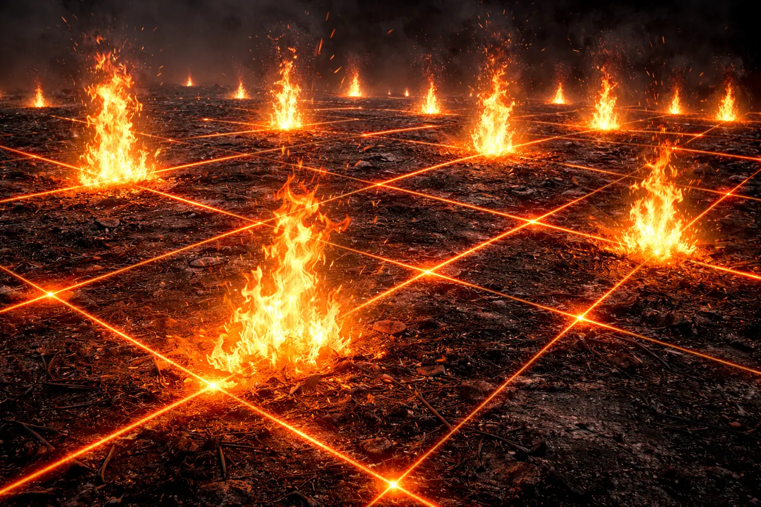
Cellular Automaton Fire Spread
Discretize landscape:
Grid cells (30-100 m resolution).
State: Unburned / Burning / Burned
Transition rules:
\[P_{\text{ignite}} = f(\text{fuel, weather, distance, time})\]Simplified:
\[P = P_0 \times \exp\left(-\frac{d}{ROS \times \Delta t}\right)\]Where:
- $P$ = ignition probability
- $P_0$ = base probability
- $d$ = distance to burning cell
- $ROS$ = rate of spread
- $\Delta t$ = time step
Algorithm:
For each time step:
  For each burning cell:
    For each neighbor:
      Calculate P_ignite
      If random() < P_ignite:
        Ignite neighbor
  Burning cells → Burned
Advantages:
- Computationally fast
- Handles complex landscapes
- Stochastic variation
Disadvantages:
- Requires calibration
- Less physical basis than Rothermel
Fire Arrival Time
Minimum time path:
\[T(x,y) = \min_{\text{path}} \int_{\text{path}} \frac{ds}{ROS(s)}\]Where:
- $T$ = arrival time
- $ds$ = path element
- $ROS(s)$ = rate of spread along path
Solved by:
Level-set methods or Dijkstra’s algorithm on grid.
Isochrones:
Contours of equal arrival time.
4. Worked Example by Hand
Problem: Calculate fire spread and perimeter.
Conditions:
- Fuel: Grass (short, dry)
- Fuel load: 0.5 kg/m²
- Fuel moisture: 6%
- Wind speed: 30 km/h (8.3 m/s)
- Slope: 15° downwind
- Initial ignition: Point source
Constants (grass fuel model):
- $\xi = 0.4$ (propagating flux ratio)
- $\epsilon = 0.7$ (effective heating)
- $Q_{ig} = 300$ kJ/kg (heat of preignition)
- $h = 18,600$ kJ/kg (heat content)
Calculate ROS, fire perimeter after 1 hour.
Solution
Step 1: Wind coefficient
Simplified: $\Phi_w \approx 0.15 U^{1.5}$ where $U$ in m/s
\[\Phi_w = 0.15 \times 8.3^{1.5} = 0.15 \times 23.9 = 3.6\]Step 2: Slope coefficient
\[\Phi_s = 5.275 \times (0.01)^{-0.3} \times \tan^2(15°)\] \[= 5.275 \times 2.15 \times 0.072 = 0.82\]Step 3: Reaction intensity
Assume $\Gamma’ = 15$ min⁻¹ (typical grass):
\[I_R = 15 \times 0.5 \times 18600 = 139,500 \text{ kW/m}^2\]Step 4: Rate of spread
\[ROS = \frac{139500 \times 0.4 \times (1 + 3.6 + 0.82)}{500 \times 0.7 \times 300}\] \[= \frac{139500 \times 0.4 \times 5.42}{105000}\] \[= \frac{302,472}{105000} = 2.88 \text{ m/min}\]Head fire ROS = 2.88 m/min = 173 m/h
Step 5: Backing fire
Assume $ROS_b = 0.1 \times ROS_h = 0.29$ m/min
Step 6: Ellipse parameters
\[a = \frac{2.88 + 0.29}{2} = 1.59 \text{ m/min}\]Length-to-breadth ratio $LB = 3$:
\[b = \frac{1.59}{3} = 0.53 \text{ m/min}\]Step 7: Perimeter after 1 hour
Semi-axes at $t = 60$ min:
\[a_{60} = 1.59 \times 60 = 95.4 \text{ m}\] \[b_{60} = 0.53 \times 60 = 31.8 \text{ m}\]Area:
\[A = \pi \times 95.4 \times 31.8 = 9,540 \text{ m}^2 \approx 1 \text{ hectare}\]Fire spread 95 m downwind, 32 m on flanks in 1 hour.
Step 8: Fireline intensity (head)
\[I = 18600 \times 0.5 \times \frac{2.88}{60} = 446 \text{ kW/m}\]Flame length:
\[L = 0.0775 \times 446^{0.46} = 0.0775 \times 12.3 = 0.95 \text{ m}\]Moderate intensity (direct attack still possible if resources available quickly)
5. Computational Implementation
Below is an interactive fire spread simulator.
Head ROS: -- m/min
Fire area: -- ha
Fireline intensity: -- kW/m
Suppression: --
Observations:
- Fire spreads fastest downwind (head fire)
- Elliptical shape elongated in wind direction
- Higher wind dramatically increases spread rate
- Slope amplifies spread when aligned with wind
- Low moisture enables rapid spread
- Fireline intensity determines suppression feasibility
Key insights:
- Exponential area growth over time
- Wind and slope effects multiplicative
- Even moderate winds create elongated fires
- Suppression window closes quickly with high intensity
6. Interpretation
Operational Fire Prediction
FARSITE workflow:
- Initialize: Ignition point, time, weather
- Propagate: Calculate ROS at fire perimeter
- Advance: Move perimeter based on ROS, timestep
- Repeat: Until forecast end or fire containment
Outputs:
- Fire perimeter evolution (hourly)
- Arrival time maps
- Intensity maps
- Flame length maps
Used for:
- Evacuation planning
- Resource pre-positioning
- Backfire/burnout strategy
- Structure triage
Example - 2018 Camp Fire (California):
FARSITE predicted Paradise threatened within 6 hours.
Enabled evacuation (though still 85 deaths, rapid spread).
Prescribed Burn Planning
Objective: Reduce fuel loads safely.
Model used to:
Determine burn window (weather conditions for control).
Required:
- Low intensity (< 1000 kW/m)
- Slow spread (< 1 m/min)
- Favorable wind direction (away from structures)
Example conditions:
- Fuel MC: 12-15%
- Wind: 10-15 km/h
- Atmospheric stability: Stable
- RH: 40-60%
Model confirms burn will remain controllable.
Post-Fire Analysis
Reconstruct fire behavior:
Given final perimeter, weather records.
Calibrate models:
Adjust parameters (fuel models, moisture, wind reduction factors).
Improve predictions:
Better local fuel characterization.
Identify extreme fire behavior:
Rates of spread » model predictions indicate:
- Spotting (long-range ember transport)
- Crown fire (not surface fire)
- Fire whirls (tornadic circulation)
7. What Could Go Wrong?
Crown Fire Transition
Surface fire models (Rothermel) don’t predict crown fire.
Crown fire: Spreads through tree canopy, 10-100× faster.
Transition: Occurs when:
\[I > I_{\text{critical}}\]Critical intensity:
\[I_{\text{crit}} = \frac{(460 + 25.9 \times MC)^{3/2}}{60} \times 0.01 \times \rho_{\text{canopy}}\]Once in crown:
ROS can exceed 100 m/min (vs 2-10 m/min surface).
Solution: Van Wagner crown fire models, FIRETEC 3D physics.
Spotting Ignored
Embers travel ahead of fire front.
Distance: Function of ember size, height lofted, wind.
Model (Albini):
\[d_{\text{spot}} = f(\text{flame length, wind, terrain})\]Typically: 0.5-2 km, extreme cases 10-30 km.
Creates secondary ignitions ahead of modelled perimeter.
Catastrophic when embers land in receptive fuel.
Solution: Spotting submodels, but highly stochastic.
Fuel Heterogeneity
Models assume uniform fuel in each type.
Reality:
Variable loading, moisture, species within same classification.
Result: Under/overprediction locally.
Solution:
- Fine-scale fuel mapping (LiDAR-derived)
- Stochastic variation in parameters
Weather Forecast Uncertainty
Fire spread depends on forecast wind, temperature, humidity.
Forecast errors propagate:
10% wind error → 15% ROS error → 25% perimeter error.
Solution:
- Ensemble forecasts (multiple weather scenarios)
- Probabilistic fire prediction
8. Extension: Machine Learning Fire Spread
Data-driven approaches:
Train on historical fires (perimeter progression, weather, fuels).
Neural networks:
Input: Fuel, weather, terrain
Output: ROS or probability of burning
Advantages:
- Capture complex nonlinear relationships
- No need to specify physics
- Fast inference
Disadvantages:
- Requires large training datasets
- Difficult to extrapolate beyond training conditions
- Less interpretable than physics-based
Hybrid: Use physics model as baseline, ML for corrections.
9. Math Refresher: Ellipse Geometry
Standard Form
\[\frac{x^2}{a^2} + \frac{y^2}{b^2} = 1\]Where:
- $a$ = semi-major axis (larger)
- $b$ = semi-minor axis (smaller)
Area:
\[A = \pi a b\]Perimeter (approximate):
\[P \approx \pi (3(a+b) - \sqrt{(3a+b)(a+3b)})\]Eccentricity
\[e = \sqrt{1 - \frac{b^2}{a^2}}\]Circle: $e = 0$ ($a = b$)
Elongated: $e \to 1$ ($b \ll a$)
Fire ellipses:
Typical $e = 0.8-0.95$ (highly elongated in strong wind).
Summary
- Fire spread rate determined by fuel, weather, and topography via Rothermel equation
- Wind and slope effects multiplicative increasing spread exponentially
- Elliptical fire growth results from directional spread differences
- Fireline intensity determines suppression difficulty with threshold at 500 kW/m
- Cellular automaton models provide computationally efficient landscape-scale simulation
- Operational systems like FARSITE predict fire perimeter evolution for planning
- Applications span wildfire prediction, prescribed burn planning, post-fire analysis
- Challenges include crown fire transition, spotting, fuel heterogeneity, weather uncertainty
- Machine learning approaches complement physics-based models
- Critical tool for emergency management and firefighter safety