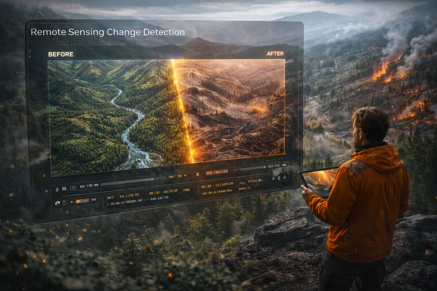
Change Detection in Satellite Imagery
Where did deforestation occur? How much urban area expanded? What burned in the wildfire? Change detection compares satellite images from different dates to map what changed. This model derives image differencing, NDVI change, change vector analysis, and post-classification comparison methods.
Prerequisites: image differencing, ratio methods, change vector analysis, thresholding
1. The Question
How much forest was lost between 2010 and 2020?
Change detection identifies where and what type of change occurred:
Applications:
- Deforestation: Forest loss mapping
- Urban growth: City expansion tracking
- Agriculture: Crop rotation patterns
- Disaster assessment: Flood/fire damage extent
- Coastal change: Erosion, land reclamation
- Mining: Excavation monitoring
Challenges:
- Phenology: Seasonal vegetation differences (not real change)
- Sensor differences: Different satellites/settings
- Atmospheric conditions: Clouds, haze, sun angle
- Registration: Images must align precisely
The mathematical question: Given two co-registered images from different dates, how do we reliably identify actual change while minimizing false positives from natural variation?
2. The Conceptual Model
Types of Change
1. Land Cover Conversion
- Forest → Urban (permanent)
- Cropland → Wetland (land use change)
2. Condition Change
- Healthy forest → Degraded forest (same class, different state)
- Dense vegetation → Sparse vegetation
3. Temporary vs. Permanent
- Snow cover (temporary)
- Deforestation (permanent)
- Crop harvest (seasonal)
Change Detection Methods
1. Image Differencing
\[\Delta = \text{Image}_2 - \text{Image}_1\]Threshold to identify significant change.
2. Image Ratioing
\[R = \frac{\text{Image}_2}{\text{Image}_1}\]Less sensitive to illumination differences.
3. NDVI Differencing
\[\Delta\text{NDVI} = \text{NDVI}_2 - \text{NDVI}_1\]Negative = vegetation loss
Positive = vegetation gain
4. Change Vector Analysis (CVA)
Compute magnitude and direction of change in multi-dimensional space.
5. Post-Classification Comparison
Classify each image independently, then compare classes:
\[\text{Change} = (\text{Class}_1 \neq \text{Class}_2)\]3. Building the Mathematical Model
Image Differencing
For band $i$:
\[\Delta_i = DN_{i,t_2} - DN_{i,t_1}\]Where $DN$ = digital number (pixel value).
Change threshold:
\[|\Delta_i| > T_i\]T can be:
- Fixed: e.g., $T = 20$ (DN units)
- Statistical: $T = k\sigma$ where $\sigma$ = standard deviation of $\Delta_i$ over stable areas
- Adaptive: Vary spatially based on local variance
Typical: $T = 2\sigma$ or $3\sigma$ (95% or 99.7% confidence)
NDVI Change Detection
NDVI at time $t$:
\[\text{NDVI}_t = \frac{\text{NIR}_t - \text{Red}_t}{\text{NIR}_t + \text{Red}_t}\]Change:
\[\Delta\text{NDVI} = \text{NDVI}_{t_2} - \text{NDVI}_{t_1}\]Interpretation:
- $\Delta\text{NDVI} < -0.2$: Significant vegetation loss (deforestation, fire)
- $-0.2 \leq \Delta\text{NDVI} < -0.1$: Moderate degradation
- $-0.1 \leq \Delta\text{NDVI} \leq 0.1$: No change (stable)
- $\Delta\text{NDVI} > 0.1$: Vegetation increase (regrowth, greening)
Advantages:
- Normalized (reduces illumination effects)
- Directly interpretable (vegetation change)
- Works across sensors
Change Vector Analysis (CVA)
Multi-band approach: Treat each pixel as vector in $n$-dimensional space.
Change vector:
\[\Delta\mathbf{x} = \mathbf{x}_{t_2} - \mathbf{x}_{t_1}\]Where $\mathbf{x} = (B_1, B_2, \ldots, B_n)$ is spectral vector.
Change magnitude:
\[M = ||\Delta\mathbf{x}|| = \sqrt{\sum_{i=1}^{n} (B_{i,t_2} - B_{i,t_1})^2}\]Change direction:
\[\theta = \arctan\left(\frac{\Delta B_2}{\Delta B_1}\right)\](For 2D case; generalizes to $n$ dimensions)
Interpretation:
- Magnitude: How much changed
- Direction: Type of change (e.g., vegetation loss vs. urban growth have different spectral trajectories)
Post-Classification Comparison
Algorithm:
1. Classify Image_t1 → Map_t1
2. Classify Image_t2 → Map_t2
3. Create change matrix:

   For each pixel (i, j):
       if Map_t1[i,j] != Map_t2[i,j]:
           Change[i,j] = type of transition
       else:
           Change[i,j] = no change
Change matrix (transition table):
| Forest_t2 | Urban_t2 | Water_t2 | |
|---|---|---|---|
| Forest_t1 | 8500 | 450 | 50 |
| Urban_t1 | 20 | 1200 | 0 |
| Water_t1 | 5 | 10 | 285 |
Analysis:
- Diagonal: No change (stable)
- Off-diagonal: Change
- 450 pixels: Forest → Urban (deforestation + urbanization)
Advantage: Provides “from-to” information
Disadvantage: Errors in both classifications compound
4. Worked Example by Hand
Problem: Detect forest loss using NDVI differencing.
Pixel values:
Date 1 (2015):
- Red = 0.08, NIR = 0.42
Date 2 (2020):
- Red = 0.25, NIR = 0.28
Solution
Step 1: Calculate NDVI for each date
Date 1:
\[\text{NDVI}_1 = \frac{0.42 - 0.08}{0.42 + 0.08} = \frac{0.34}{0.50} = 0.68\]Date 2:
\[\text{NDVI}_2 = \frac{0.28 - 0.25}{0.28 + 0.25} = \frac{0.03}{0.53} = 0.057\]Step 2: Calculate NDVI change
\[\Delta\text{NDVI} = 0.057 - 0.68 = -0.623\]Step 3: Interpret
Large negative change ($< -0.2$) → Significant vegetation loss
Likely: Deforestation or land clearing occurred between 2015 and 2020.
Original pixel: Dense vegetation (NDVI = 0.68, healthy forest)
New pixel: Bare soil or sparse vegetation (NDVI = 0.057)
Conclusion: Forest loss detected.
5. Computational Implementation
Below is an interactive change detection demo.
Total pixels: --
Changed pixels: --
Change rate: --%
Try this:
- NDVI differencing: Most sensitive to vegetation change
- Image differencing: Simple NIR band comparison
- Change vector analysis: Uses both Red and NIR together
- Adjust threshold: Higher = only major changes detected
- Show change only: Isolates just the changed areas (red/green)
- Time 1: All forest (uniformly green)
- Time 2: Clearcut region visible (less green)
- Change map: Red shows deforestation area clearly!
Key insight: Change detection reveals WHERE and HOW MUCH changed—critical for monitoring deforestation, urbanization, and disasters!
6. Interpretation
Global Forest Change
Hansen et al. (2013) Global Forest Change dataset:
- 30m resolution, 2000-2023
- Annual forest loss maps
- Based on Landsat time series
- Free, publicly available
Method: NDVI-based change detection + classification
Findings:
- ~1.5 million km² forest lost 2000-2012
- Brazil, Indonesia, Canada largest losses
- Tropics most dynamic
Urban Growth Monitoring
Nighttime lights change detection:
- VIIRS/DMSP satellite data
- Increase in lights = urbanization
- Independent of weather/season
NDVI decrease + impervious surface increase = urban expansion
Disaster Assessment
Rapid mapping after events:
Floods:
- Water extent change (NIR differencing)
- Pre-flood vs. during flood
Wildfires:
- NDVI drop in burned areas
- Burn severity mapping (dNBR)
Earthquakes:
- Building collapse (texture change)
- Landslides (slope failure)
Agricultural Monitoring
Crop rotation:
- Annual land cover change
- Corn-soybean patterns
Irrigation expansion:
- NDVI increase in arid regions
- Water use monitoring
7. What Could Go Wrong?
Phenological Differences
Images from different seasons:
Time 1: July (peak green)
Time 2: November (senescence)

Result: ΔNDVI < 0 everywhere (false change!)
Solution:
- Use anniversary dates (same month/season)
- Or normalize for phenology using time series
- Multi-year baseline to understand natural variation
Atmospheric Differences
Haze, clouds, sun angle affect reflectance.
Apparent change from atmospheric conditions, not land cover.
Solution:
- Atmospheric correction (essential!)
- Cloud masking
- Surface reflectance products (pre-corrected)
Registration Errors
Images misaligned by 1-2 pixels:
Edge pixels show false change.
Solution:
- Co-registration (align precisely)
- Sub-pixel accuracy (<0.5 pixel)
- Buffer stable features to avoid edges
Classification Error Propagation
Post-classification comparison:
If each classification is 90% accurate:
Overall accuracy of change detection ≈ $0.9 \times 0.9 = 81\%$
Errors compound!
Solution:
- Use direct change detection (differencing) when possible
- Improve individual classifications first
8. Extension: Continuous Change Detection
Traditional: Compare two dates (binary change/no-change)
Time series approach: Continuous monitoring
BFAST (Breaks For Additive Season and Trend):
Decomposes time series into:
- Trend (long-term change)
- Seasonal (phenology)
- Remainder (noise + abrupt changes)
Detects:
- Gradual change (forest degradation)
- Abrupt change (clearcut)
- Timing of change (when it occurred)
LandTrendr (Landsat-based Detection of Trends in Disturbance and Recovery):
Fits segmented trajectories to NDVI time series:
- Growth (reforestation)
- Decline (degradation)
- Stable (no change)
Advantage: Richer information than two-date comparison
9. Math Refresher: Statistical Thresholding
Normal Distribution Assumption
If $\Delta$ values for “no change” pixels follow normal distribution:
\[\Delta \sim N(0, \sigma^2)\]Change threshold:
\[T = \mu + k\sigma\]Where:
- $\mu$ = mean (ideally 0 for radiometric correction)
- $\sigma$ = standard deviation
- $k$ = 2 (95% confidence) or 3 (99.7% confidence)
Estimating σ from Data
Use stable areas (known no-change):
1. Identify stable regions (water, urban cores)
2. Calculate Δ for these pixels
3. Estimate σ = std(Δ_stable)
4. Set T = k*σ
ROC Analysis
Receiver Operating Characteristic:
Plot True Positive Rate vs. False Positive Rate for different thresholds.
Optimal threshold: Maximize TPR while minimizing FPR
Area Under Curve (AUC): Measure of classifier quality
- AUC = 1.0: Perfect
- AUC = 0.5: Random
Summary
- Change detection identifies where land cover changed between two dates
- Image differencing: Simple subtraction, threshold for significant change
- NDVI differencing: Normalized, reduces illumination effects, vegetation-specific
- Change vector analysis (CVA): Multi-band magnitude and direction
- Post-classification comparison: Provides from-to change matrix
- Threshold selection: 2-3 standard deviations from stable area variation
- Applications: Deforestation, urban growth, disaster assessment, agriculture
- Challenges: Phenology, atmosphere, registration errors, classification error propagation
- Time series methods: BFAST, LandTrendr for continuous monitoring
- Critical for environmental monitoring and reporting (e.g., REDD+, SDG indicators)