modelling Level 3

Carbon Allocation and Net Primary Productivity

Photosynthesis fixes carbon. But not all of it becomes biomass—plants burn carbon for energy (respiration), and allocate the remainder among leaves, stems, and roots. This model models carbon flow from GPP through allocation to NPP, and tracks biomass accumulation in different plant pools.

Prerequisites: carbon balance, allocation coefficients, turnover rates, pool dynamics

26 Feb 2026 Updated 12 Mar 2026 12 min read

1. The Question

Where does the carbon go after photosynthesis fixes it?

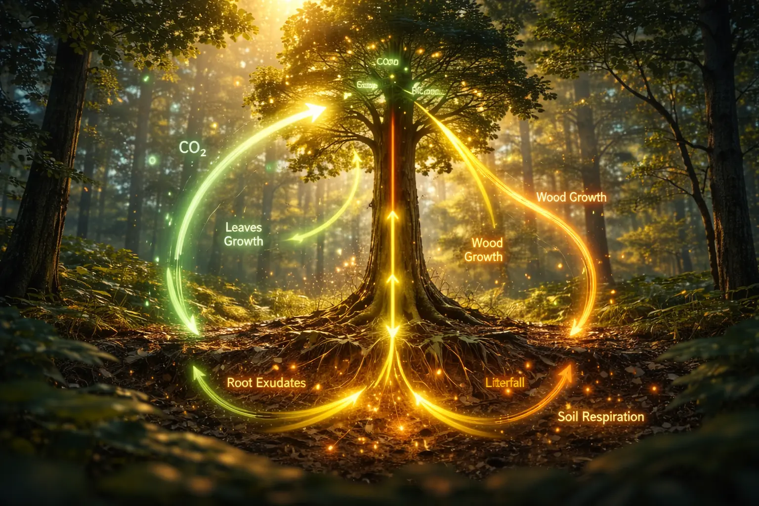
A forest canopy captures sunlight and converts CO₂ to sugars (Gross Primary Productivity, GPP). But the forest uses carbon for:

Maintaining existing tissues — respiring sugars for energy
Building new leaves — to capture more light
Growing roots — to access water and nutrients
Adding wood — structural support and long-term storage

The difference between carbon fixed (GPP) and carbon burned (respiration) is Net Primary Productivity (NPP) — the actual carbon available for growth.

The mathematical question: How do we model carbon flow from GPP to biomass pools, accounting for respiration and turnover?

2. The Conceptual Model

Carbon Flow in Ecosystems

Gross Primary Productivity (GPP):
Total carbon fixed by photosynthesis (Model 20).

Autotrophic Respiration ($R_a$):
Carbon burned by plants for energy (maintenance + growth respiration).

Net Primary Productivity (NPP):

\[\text{NPP} = \text{GPP} - R_a\]

Carbon Allocation:
NPP is allocated among plant parts:

Leaves (foliage): $a_L \times \text{NPP}$
Stems (wood): $a_S \times \text{NPP}$
Roots: $a_R \times \text{NPP}$

Where $a_L + a_S + a_R = 1$ (allocation fractions sum to 1).

Biomass Pools:
Each pool accumulates carbon but also loses it through turnover (death, litterfall).

\[\frac{dC_L}{dt} = a_L \cdot \text{NPP} - k_L C_L\]

Where:

$C_L$ = leaf carbon (kg C/m²)
$k_L$ = turnover rate (year⁻¹)

Respiration Components

Maintenance respiration ($R_m$):
Energy to maintain existing tissues (proportional to biomass).

\[R_m = r_m (C_L + C_S + C_R)\]

Where $r_m$ is specific maintenance rate (kg C respired per kg C biomass per year).

Growth respiration ($R_g$):
Energy cost of synthesizing new tissue (proportional to NPP).

\[R_g = r_g \cdot (GPP - R_m)\]

Where $r_g$ is growth respiration fraction (typically 0.2–0.3).

Total autotrophic respiration:

\[R_a = R_m + R_g = R_m + r_g(\text{GPP} - R_m)\]

Solve for $R_a$:

\[R_a = \frac{R_m + r_g \cdot \text{GPP}}{1 + r_g}\]

3. Building the Mathematical Model

Three-Pool Carbon Model

State variables:

$C_L$ = leaf carbon (kg C/m²)
$C_S$ = stem (wood) carbon (kg C/m²)
$C_R$ = root carbon (kg C/m²)

Dynamics:

\[\frac{dC_L}{dt} = a_L \cdot \text{NPP} - k_L C_L\] \[\frac{dC_S}{dt} = a_S \cdot \text{NPP} - k_S C_S\] \[\frac{dC_R}{dt} = a_R \cdot \text{NPP} - k_R C_R\]

Turnover rates (typical values):

Leaves: $k_L = 1$ year⁻¹ (leaves live 1 year average)
Fine roots: $k_R = 1$ year⁻¹ (similar to leaves)
Wood: $k_S = 0.02$ year⁻¹ (50-year lifespan)

Allocation fractions (vary by ecosystem):

Young forest: $a_L = 0.3$, $a_S = 0.4$, $a_R = 0.3$ (building structure)
Mature forest: $a_L = 0.25$, $a_S = 0.50$, $a_R = 0.25$ (less leaf, more wood)
Grassland: $a_L = 0.4$, $a_S = 0.0$, $a_R = 0.6$ (no wood, deep roots)

Steady State

At equilibrium (mature ecosystem):

\[\frac{dC_L}{dt} = 0 \implies C_L^* = \frac{a_L \cdot \text{NPP}}{k_L}\]

Example: NPP = 1 kg C/m²/year, $a_L = 0.3$, $k_L = 1$ year⁻¹:

\[C_L^* = \frac{0.3 \times 1}{1} = 0.3 \text{ kg C/m}^2\]

Total steady-state carbon:

\[C_{\text{total}}^* = \frac{a_L}{k_L} \text{NPP} + \frac{a_S}{k_S} \text{NPP} + \frac{a_R}{k_R} \text{NPP}\] \[= \text{NPP} \left(\frac{a_L}{k_L} + \frac{a_S}{k_S} + \frac{a_R}{k_R}\right)\]

Wood dominates because $k_S$ is small (low turnover).

4. Worked Example by Hand

Problem: A temperate forest has:

GPP = 2.5 kg C/m²/year
Maintenance respiration: $R_m = 0.8$ kg C/m²/year
Growth respiration fraction: $r_g = 0.25$
Allocation: $a_L = 0.25$, $a_S = 0.50$, $a_R = 0.25$
Turnover: $k_L = 1$, $k_S = 0.02$, $k_R = 1$ year⁻¹

(a) Calculate NPP.
(b) Find steady-state carbon in each pool.
(c) What is total ecosystem carbon at equilibrium?

Solution

(a) NPP

\[R_a = \frac{R_m + r_g \cdot \text{GPP}}{1 + r_g} = \frac{0.8 + 0.25 \times 2.5}{1 + 0.25}\] \[= \frac{0.8 + 0.625}{1.25} = \frac{1.425}{1.25} = 1.14 \text{ kg C/m}^2\text{/year}\] \[\text{NPP} = \text{GPP} - R_a = 2.5 - 1.14 = 1.36 \text{ kg C/m}^2\text{/year}\]

(b) Steady-state carbon

Leaves:

\[C_L^* = \frac{a_L \cdot \text{NPP}}{k_L} = \frac{0.25 \times 1.36}{1} = 0.34 \text{ kg C/m}^2\]

Stems:

\[C_S^* = \frac{a_S \cdot \text{NPP}}{k_S} = \frac{0.50 \times 1.36}{0.02} = \frac{0.68}{0.02} = 34 \text{ kg C/m}^2\]

Roots:

\[C_R^* = \frac{a_R \cdot \text{NPP}}{k_R} = \frac{0.25 \times 1.36}{1} = 0.34 \text{ kg C/m}^2\]

(c) Total carbon

\[C_{\text{total}}^* = 0.34 + 34 + 0.34 = 34.68 \text{ kg C/m}^2\]

Interpretation: Wood (stems) stores 98% of total carbon, even though only 50% of NPP goes to wood. This is because wood lives ~50 years while leaves/roots live ~1 year.

Convert to biomass: Assuming carbon is ~50% of dry biomass:

\[\text{Biomass} = \frac{34.68}{0.5} = 69.4 \text{ kg dry mass/m}^2 = 694 \text{ tonnes/ha}\]

Typical for a mature temperate forest.

5. Computational Implementation

Below is an interactive carbon allocation simulator.

Ecosystem type: GPP (kg C/m²/year): 2.5 Leaf allocation (aL): 0.25 Wood allocation (aS): 0.50 Simulation years: 100 years

NPP: kg C/m²/year

R_a/GPP:

Final total carbon: kg C/m²

Equilibrium reached:

Try this:

Young forest: Higher wood allocation → rapid stem growth
Mature forest: Stem carbon accumulates to ~30-40 kg C/m² over 100 years
Grassland: No wood allocation → only leaves and roots, reaches equilibrium quickly
Cropland: Annual harvest (high turnover) → low steady-state carbon
Increase GPP: More NPP → faster accumulation
Notice: Stems take decades to reach equilibrium (slow turnover), leaves equilibrate in ~2-3 years

Key insight: Long-lived pools (wood) dominate ecosystem carbon storage, even if allocation is similar to short-lived pools.

6. Interpretation

Forest Carbon Sequestration

Young forest (0–50 years):

Rapid growth
NPP high
Carbon accumulation ~0.5–2 kg C/m²/year
Carbon sink

Mature forest (> 100 years):

Near equilibrium
Growth balanced by mortality
NPP still positive but slower accumulation
Weak carbon sink or neutral

Old-growth debate: Do old forests continue to sequester carbon?
Evidence suggests some continued net uptake (~0.1–0.2 kg C/m²/year).

NPP/GPP Ratio

Carbon use efficiency:

\[\text{CUE} = \frac{\text{NPP}}{\text{GPP}}\]

Typical values:

Young forest: 0.60 (low respiration costs)
Mature forest: 0.50 (higher maintenance from large biomass)
Stressed ecosystem: 0.30 (high respiration, drought, heat)

Global average: CUE ≈ 0.47 (forests), 0.55 (grasslands), 0.60 (croplands)

Harvest and Regrowth

Clear-cut harvest:

Removes most aboveground biomass ($C_L$, $C_S$)
Roots partially remain ($C_R$)
Regrowth from sprouts/seeds
Carbon rebounds over 20–50 years

modelling:
Reset $C_L = 0.1$, $C_S = 0.1$, keep $C_R$ reduced, simulate regrowth.

7. What Could Go Wrong?

Assuming Constant Allocation

Real allocation changes with:

Tree age: Young trees allocate more to leaves/roots, mature trees to wood
Resource availability: Nutrient-limited → more roots, light-limited → more leaves
CO₂ fertilization: Elevated CO₂ may shift allocation toward roots

Dynamic allocation models: Make $a_L$, $a_S$, $a_R$ functions of resource status.

Ignoring Litterfall Fate

Dead leaves/roots don’t disappear—they become soil organic matter (SOM).

Complete carbon cycle:

\[\text{GPP} \to \text{NPP} \to \text{Biomass} \to \text{Litter} \to \text{SOM} \to \text{Respiration (decomposition)}\]

Our model stops at biomass. Full model needs soil carbon pools (next-level complexity).

Constant Turnover Rates

Turnover varies with:

Temperature: Faster decomposition in tropics
Moisture: Slow in deserts (dry) and peat bogs (waterlogged)
Disturbance: Fire, insects, disease accelerate mortality

Q₁₀ rule: Decomposition doubles per 10°C warming.

Neglecting Allocation to Reproduction

Plants allocate carbon to seeds, flowers, fruits—our model lumps this into “leaves” or ignores it.

For crops: Grain yield is a separate allocation pool.

8. Extension: Net Ecosystem Productivity

Net Ecosystem Productivity (NEP):

\[\text{NEP} = \text{NPP} - R_h\]

Where $R_h$ is heterotrophic respiration (decomposition of dead organic matter by microbes).

NEP > 0: Ecosystem is a carbon sink
NEP < 0: Ecosystem is a carbon source
NEP ≈ 0: Ecosystem at steady state

Global NEP:
Terrestrial ecosystems sequester ~2–3 Pg C/year (about 1/4 of fossil fuel emissions).

Next model will shift to atmospheric interactions—wind profiles and turbulent mixing that transport heat, moisture, and CO₂ between surface and atmosphere.

9. Math Refresher: Compartment Models

General Form

A multi-compartment model has:

State variables: $C_1, C_2, …, C_n$ (pool sizes)
Flows: $F_{ij}$ from pool $i$ to pool $j$
Inputs/outputs: External sources/sinks

\[\frac{dC_i}{dt} = \sum_j F_{ji} - \sum_j F_{ij}\]

Matrix Representation

For linear flows ($F_{ij} = k_{ij} C_i$):

\[\frac{d\mathbf{C}}{dt} = \mathbf{A} \mathbf{C} + \mathbf{u}\]

Where:

$\mathbf{C}$ = vector of pool sizes
$\mathbf{A}$ = transfer matrix
$\mathbf{u}$ = input vector

Steady state: $\mathbf{A} \mathbf{C}^* + \mathbf{u} = 0$

Our model:

\[\mathbf{C} = \begin{pmatrix} C_L \\ C_S \\ C_R \end{pmatrix}, \quad \mathbf{A} = \begin{pmatrix} -k_L & 0 & 0 \\ 0 & -k_S & 0 \\ 0 & 0 & -k_R \end{pmatrix}, \quad \mathbf{u} = \text{NPP} \begin{pmatrix} a_L \\ a_S \\ a_R \end{pmatrix}\]

Summary

NPP = GPP - autotrophic respiration (carbon available for growth)
Autotrophic respiration has two components: maintenance + growth
Carbon allocation: NPP distributed among leaves, stems, roots
Biomass dynamics: Each pool accumulates new growth and loses carbon through turnover
Turnover rates: Fast for leaves/roots (~1 year), slow for wood (~50 years)
Steady state: Pool size = (allocation × NPP) / turnover rate
Wood dominates ecosystem carbon despite similar allocation because of low turnover
Carbon use efficiency (NPP/GPP) typically 0.4–0.6
Young forests are strong carbon sinks; mature forests approach equilibrium