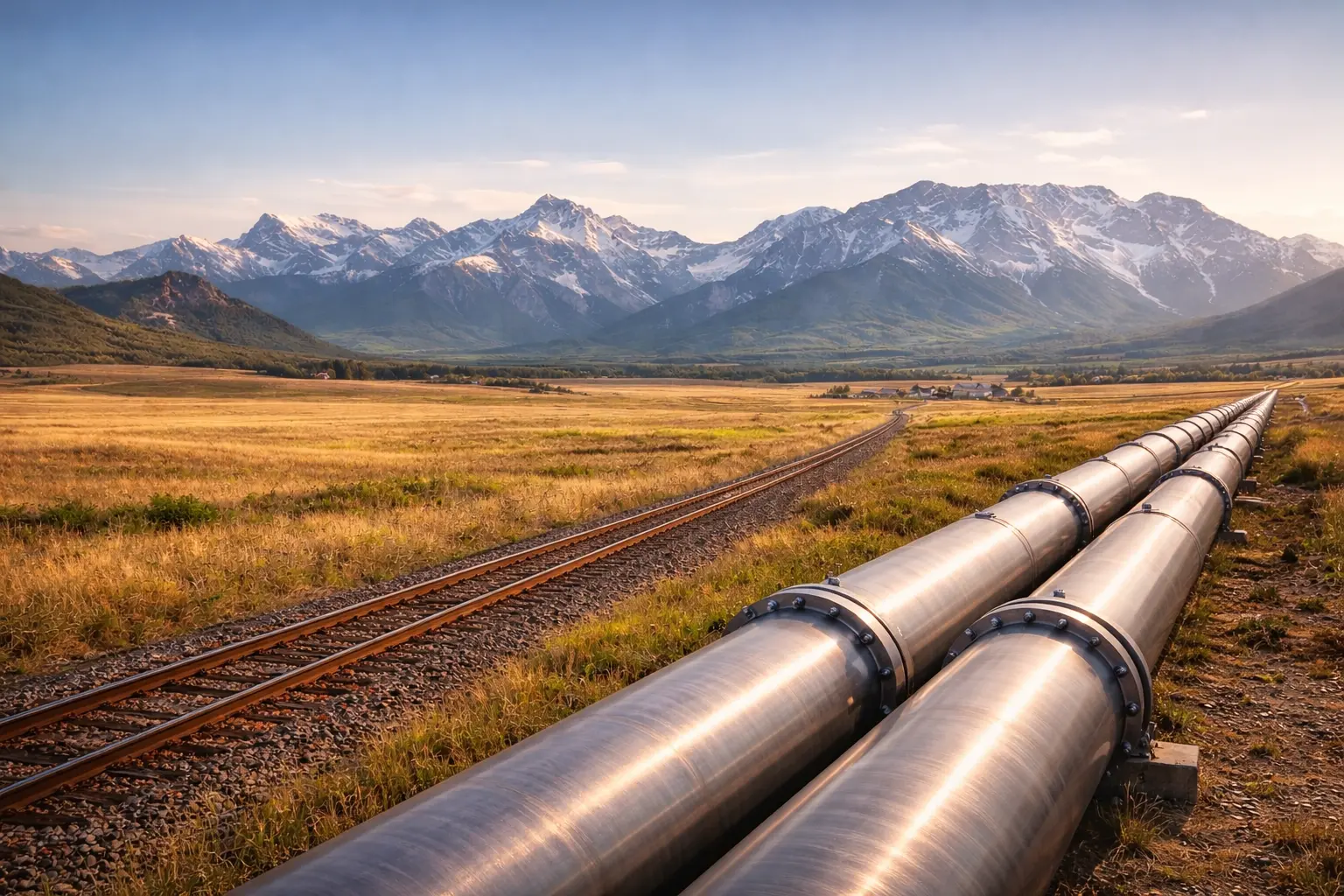
NGL and Condensate Pipeline Systems
Every barrel of diluted bitumen leaving Alberta requires roughly 0.3 barrels of diluent to make it flow. That diluent — mostly condensate — travels north from U.S. gas plays and Alberta's own deep-cut gas plants through a largely invisible pipeline system. NGL infrastructure is the circulatory system beneath Alberta's oil sands economy.
Prerequisites: Phase equilibria (conceptual), mass balance, fractionation yield ratios
1. The Question
What keeps diluted bitumen flowing, and where does the diluent come from?
Essay P1 established that Alberta exports approximately 3.5 million barrels per day of crude oil — mostly diluted bitumen. But dilbit is a blend. Roughly 70% is bitumen; the remaining 30% is condensate or synthetic crude added to reduce viscosity enough for pipeline transport. That diluent has to come from somewhere, travel to the oil sands by pipeline, get blended, travel south with the bitumen, and then — at the destination refinery — be separated and either used locally or returned north.
The infrastructure that handles this — the natural gas liquids (NGL) gathering systems, fractionators, and condensate pipelines — is less visible in public debate than the crude trunk lines. It is no less essential. Without a functioning diluent supply chain, oil sands bitumen cannot move.
This essay maps the NGL and condensate systems, derives the mass balance mathematics of the fractionation cascade, and traces the geographic logic of why condensate flows north while bitumen flows south.
2. The Conceptual Model
What natural gas liquids are
When natural gas is produced from the ground, it contains methane (the dominant component) plus heavier hydrocarbon molecules that are gaseous at reservoir pressure but can be condensed to liquid at surface conditions. These heavier molecules are natural gas liquids:
| Component | Formula | Boiling Point | Primary Use |
|---|---|---|---|
| Ethane | C₂H₆ | −89°C | Ethylene cracking (plastics) |
| Propane | C₃H₈ | −42°C | Heating, petrochemical feedstock |
| Butane | C₄H₁₀ | −1°C | Blending, feedstock |
| Pentane+ (condensate) | C₅H₁₂+ | 36°C+ | Diluent for bitumen |
NGLs are extracted from the raw gas stream at gas plants using a process called deep-cut extraction — chilling the gas until the heavier components condense out. The resulting mixture of NGLs is called raw mix or y-grade, and it travels by pipeline to a fractionator, which separates it into individual products using distillation.
The pentane-plus fraction — condensate — is the critical link to the oil sands. It is the lightest liquid hydrocarbon, mixes readily with bitumen, and reduces viscosity sufficiently to allow pipeline transport.
The diluent circuit
The diluent supply chain forms a circuit with a counterintuitive geography:
- Condensate is produced in deep-cut gas plants across the WCSB (Western Canadian Sedimentary Basin) and imported from U.S. sources via the reversed Cochin pipeline
- Condensate travels north to Hardisty, Fort Saskatchewan, and oil sands blending terminals near Fort McMurray
- Bitumen is blended with condensate (~70/30 ratio by volume) to produce dilbit
- Dilbit travels south through the crude trunk system (Essay P1)
- At destination refineries, the condensate is separated from the bitumen and either used locally or shipped back north
This means the crude pipeline system and the condensate/NGL system are not independent — they are coupled. A constraint on condensate supply directly limits oil sands production volume, regardless of how much crude export capacity exists.
The Cochin reversal: a case study in adaptive infrastructure
The Cochin pipeline — 2,900 km long, running originally from Fort Saskatchewan, Alberta to Windsor, Ontario — was built in 1978 to carry propane and ethane eastward. In 2014, Kinder Morgan reversed the direction of Cochin’s northern segment, converting it to carry condensate northward from Kankakee, Illinois to Hardisty, Alberta.
This reversal added approximately 95,000 bbl/d of condensate import capacity into Alberta — supply that originates primarily from Bakken and Marcellus gas processing, making U.S. shale production a structural input to Alberta’s oil sands output. The geographic interdependence runs in both directions across the border.
Fort Saskatchewan: the fractionation hub
The Industrial Heartland northeast of Edmonton — centred on Fort Saskatchewan — contains the largest concentration of hydrocarbon fractionation capacity in Canada. The main fractionators there include:
- Inter Pipeline Empress fractionators (three trains, combined ~200,000 bbl/d NGL throughput)
- Gibson Energy’s Hardisty terminal (condensate blending, storage)
- Keyera Fort Saskatchewan (ethane, propane, butane fractionation)
- Pembina’s Redwater complex (propane and condensate fractionation)
- Dow Chemical / Nova Chemicals ethane crackers (consuming ethane from the NGL stream to make ethylene and polyethylene)
This concentration of processing infrastructure is geographically determined: Fort Saskatchewan sits at the junction of WCSB gas gathering systems, the crude mainline system, and the petrochemical corridor along the North Saskatchewan River.
3. The Mathematical Model
Mass balance through a fractionator
A fractionator takes a raw NGL mix feed and separates it into component streams. The fundamental constraint is mass conservation. If we define the feed composition as a vector of mole fractions $\mathbf{z}$, and the recovery of each component $i$ into the overhead or bottoms stream as $r_i$, then the product flow rates are:
\[F_i = F_{\text{feed}} \cdot z_i \cdot r_i\]where:
- $F_i$ is the flow rate of component $i$ in the product stream (m³/d or bbl/d, converted from molar units using component densities)
- $F_{\text{feed}}$ is the total feed flow rate
- $z_i$ is the mole fraction of component $i$ in the feed
- $r_i$ is the recovery fraction for component $i$ (0–1)
The total mass balance requires:
\[F_{\text{feed}} \cdot \rho_{\text{feed}} = \sum_i F_i \cdot \rho_i\]where $\rho$ denotes density. Because component densities differ, volume is not conserved — mass is. Ethane is less dense than propane, which is less dense than condensate, so the volumetric sum of products differs slightly from the volumetric feed.
Diluent requirement for dilbit production
For a target dilbit viscosity suitable for pipeline transport, the blending ratio is approximately:
\[\text{Blend ratio} = \frac{V_{\text{diluent}}}{V_{\text{bitumen}}} \approx 0.30 \text{ to } 0.35\]The diluent requirement for a given bitumen production rate is therefore:
\[V_{\text{diluent}} = V_{\text{bitumen}} \times r_{\text{blend}}\]where $r_{\text{blend}}$ is the volumetric blend ratio. For Alberta’s total bitumen production of approximately 3.3 million bbl/d:
\[V_{\text{diluent}} \approx 3{,}300{,}000 \times 0.30 \approx 990{,}000 \text{ bbl/d}\]Approximately 1 million barrels per day of condensate and other diluent is required to transport Alberta’s bitumen output. This is itself a larger volume than the entire crude output of many oil-producing nations.
The yield ratio and fractionation economics
For a gas plant processing raw gas with a given NGL content, the yield of each NGL component per unit of raw gas is a key economic parameter:
\[Y_i = \frac{V_i \text{ (litres of component } i \text{ recovered)}} {V_{\text{gas}} \text{ (10}^3 \text{ m}^3 \text{ of raw gas processed)}}\]Typical WCSB deep-cut plant yields (litres per 10³ m³ of raw gas):
| Component | Typical Yield (L/10³m³) |
|---|---|
| Ethane | 15–25 |
| Propane | 12–20 |
| Butane | 5–9 |
| Condensate (C5+) | 8–20 |
These yields determine the total NGL production available from a gas basin and therefore constrain the maximum diluent supply from domestic sources.
4. Worked Example by Hand
How much condensate does Cochin deliver annually, and is it enough?
Cochin’s northbound capacity (Kankakee to Hardisty): 95,000 bbl/d
Step 1 — Annual volume:
\[V_{\text{Cochin}} = 95{,}000 \text{ bbl/d} \times 365 = 34{,}675{,}000 \text{ bbl/yr}\]Step 2 — As a fraction of total diluent requirement:
Alberta’s total diluent requirement (at 3.3 Mbbl/d bitumen, 30% blend): \(V_{\text{diluent, total}} = 990{,}000 \text{ bbl/d}\)
Cochin’s share: \(\text{Cochin fraction} = \frac{95{,}000}{990{,}000} \approx 9.6\%\)
Cochin supplies roughly one-tenth of Alberta’s total diluent requirement. The remainder comes from:
- WCSB deep-cut gas plants (largest source, ~55%)
- Synthetic crude blending (bitumen blended with SCO rather than condensate, ~20%)
- Other import routes and storage drawdowns (~15%)
Step 3 — Mass balance through a representative fractionator:
Suppose a Fort Saskatchewan fractionator receives 50,000 bbl/d of raw NGL mix with the following approximate composition:
| Component | Mole fraction $z_i$ | Recovery $r_i$ | Product flow (bbl/d) |
|---|---|---|---|
| Ethane | 0.28 | 0.92 | 12,880 |
| Propane | 0.32 | 0.97 | 15,520 |
| Butane | 0.18 | 0.98 | 8,820 |
| Condensate (C5+) | 0.22 | 0.99 | 10,890 |
Note: these are mole fractions, not volume fractions. The volumetric conversion requires component densities; for this worked example we use approximate volumetric equivalents for illustrative purposes.
Total condensate yield: ~10,890 bbl/d from this single fractionator. At 15 fractionation trains across the Fort Saskatchewan Heartland, total condensate output of the order of 150,000–200,000 bbl/d enters the diluent supply chain from local processing alone.
Step 4 — Diluent value:
At a condensate price of approximately USD $55/bbl (roughly WTI less a $20 quality discount, converted at 0.73 CAD/USD):
\[P_{\text{condensate, CAD}} = \frac{55}{0.73} \approx \$75.3 \text{ CAD/bbl}\]Annual value of Cochin’s 95,000 bbl/d: \(V = 95{,}000 \times 365 \times 75.3 \approx \$2.61 \text{ billion CAD/yr}\)
A single condensate import pipeline represents over $2.6 billion in annual input supply to the oil sands industry.
5. Computational Implementation
# Foundation Implementation
# NGL fractionation mass balance and diluent supply calculator

# Component properties (approximate, for WCSB typical streams)
COMPONENTS = {
    "ethane":     {"mw": 30.07,  "density_kg_m3": 356,  "price_cad_bbl": 12.0},
    "propane":    {"mw": 44.10,  "density_kg_m3": 507,  "price_cad_bbl": 42.0},
    "butane":     {"mw": 58.12,  "density_kg_m3": 584,  "price_cad_bbl": 55.0},
    "condensate": {"mw": 86.00,  "density_kg_m3": 690,  "price_cad_bbl": 75.0},
}

BBL_TO_M3 = 0.158987

def fractionator_mass_balance(feed_bbl_d: float,
                               feed_composition: dict,
                               recovery: dict) -> dict:
    """
    Simple fractionator mass balance.

    Parameters
    ----------
    feed_bbl_d       : total feed flow rate in bbl/d
    feed_composition : dict of component -> mole fraction (must sum to 1)
    recovery         : dict of component -> recovery fraction (0-1)

    Returns
    -------
    dict of component -> product flow in bbl/d (approximate volumetric)
    """
    assert abs(sum(feed_composition.values()) - 1.0) < 0.001, \
        "Feed composition must sum to 1.0"

    results = {}
    for comp, z in feed_composition.items():
        r = recovery.get(comp, 0.95)
        # Approximate: treat mole fraction ≈ volume fraction for illustration
        results[comp] = feed_bbl_d * z * r

    return results

def diluent_requirement(bitumen_bbl_d: float,
                         blend_ratio: float = 0.30) -> float:
    """Condensate/diluent required to transport a given bitumen volume."""
    return bitumen_bbl_d * blend_ratio

def dilbit_volume(bitumen_bbl_d: float, blend_ratio: float = 0.30) -> float:
    """Total dilbit volume (bitumen + diluent)."""
    return bitumen_bbl_d + diluent_requirement(bitumen_bbl_d, blend_ratio)

# --- Alberta-scale diluent analysis ---
ALBERTA_BITUMEN_BBL_D = 3_300_000
BLEND_RATIO = 0.30

diluent_needed = diluent_requirement(ALBERTA_BITUMEN_BBL_D, BLEND_RATIO)
dilbit_total = dilbit_volume(ALBERTA_BITUMEN_BBL_D, BLEND_RATIO)

print("=== Alberta Diluent Supply Chain ===\n")
print(f"  Bitumen production          : {ALBERTA_BITUMEN_BBL_D:>12,} bbl/d")
print(f"  Blend ratio (diluent/total) : {BLEND_RATIO:.0%}")
print(f"  Diluent required            : {diluent_needed:>12,.0f} bbl/d")
print(f"  Total dilbit export volume  : {dilbit_total:>12,.0f} bbl/d")

print(f"\n  Diluent supply sources (approximate):")
sources = {
    "WCSB deep-cut gas plants":   0.55,
    "SCO as diluent (upgraders)": 0.20,
    "Cochin pipeline (import)":   0.096,
    "Other imports / storage":    0.154,
}
for source, share in sources.items():
    vol = diluent_needed * share
    print(f"    {source:<35}: {vol:>8,.0f} bbl/d  ({share:.1%})")

# --- Fractionator worked example ---
print(f"\n=== Fort Saskatchewan Fractionator: Mass Balance ===\n")

feed = 50_000  # bbl/d
composition = {"ethane": 0.28, "propane": 0.32, "butane": 0.18, "condensate": 0.22}
recovery    = {"ethane": 0.92, "propane": 0.97, "butane": 0.98, "condensate": 0.99}

products = fractionator_mass_balance(feed, composition, recovery)

print(f"  Feed: {feed:,} bbl/d raw NGL mix\n")
print(f"  {'Component':<15} {'Flow (bbl/d)':>13} {'Value (CAD/d)':>14}")
print(f"  {'-'*44}")
total_value = 0
for comp, flow in products.items():
    price = COMPONENTS[comp]["price_cad_bbl"]
    value = flow * price
    total_value += value
    print(f"  {comp:<15} {flow:>13,.0f} {value:>14,.0f}")
print(f"  {'-'*44}")
print(f"  {'TOTAL':<15} {sum(products.values()):>13,.0f} {total_value:>14,.0f}")
print(f"\n  Daily revenue: CAD ${total_value:,.0f}")
print(f"  Annual revenue: CAD ${total_value * 365 / 1e6:.1f}M")

# --- Cochin pipeline economics ---
print(f"\n=== Cochin Pipeline: Annual Condensate Import Value ===\n")
cochin_bbl_d = 95_000
condensate_price_cad = COMPONENTS["condensate"]["price_cad_bbl"]
annual_value = cochin_bbl_d * 365 * condensate_price_cad
print(f"  Capacity      : {cochin_bbl_d:,} bbl/d")
print(f"  Price (approx): CAD ${condensate_price_cad:.2f}/bbl")
print(f"  Annual value  : CAD ${annual_value / 1e9:.2f} billion")
print(f"  Share of diluent supply: {cochin_bbl_d / diluent_needed:.1%}")
Professional Implementation
# Professional Implementation
# NGL system: multi-train fractionation, diluent circuit, and supply security analysis

from dataclasses import dataclass, field
from typing import Optional
import math

@dataclass
class NGLComponent:
    name: str
    formula: str
    boiling_point_c: float
    density_kg_m3: float
    price_cad_bbl: float
    primary_use: str

@dataclass
class FractionatorTrain:
    name: str
    location: str
    operator: str
    feed_capacity_bbl_d: float
    feed_composition: dict   # component -> mole fraction
    recovery: dict           # component -> fraction recovered
    commissioned_year: Optional[int] = None

    def product_flows(self) -> dict:
        """Return product flow rates (bbl/d) by component."""
        return {
            comp: self.feed_capacity_bbl_d * z * self.recovery.get(comp, 0.95)
            for comp, z in self.feed_composition.items()
        }

    def condensate_yield_bbl_d(self) -> float:
        flows = self.product_flows()
        return flows.get("condensate", 0.0)

    def daily_revenue_cad(self, prices: dict) -> float:
        return sum(
            flow * prices.get(comp, 0.0)
            for comp, flow in self.product_flows().items()
        )


@dataclass
class DiluentsSupplyChain:
    """Model the diluent supply and demand balance for Alberta oil sands."""
    bitumen_production_bbl_d: float
    blend_ratio: float = 0.30
    fractionator_trains: list[FractionatorTrain] = field(default_factory=list)
    import_pipelines: dict = field(default_factory=dict)  # name -> bbl/d

    @property
    def diluent_demand_bbl_d(self) -> float:
        return self.bitumen_production_bbl_d * self.blend_ratio

    @property
    def dilbit_volume_bbl_d(self) -> float:
        return self.bitumen_production_bbl_d * (1 + self.blend_ratio)

    @property
    def domestic_condensate_supply_bbl_d(self) -> float:
        return sum(t.condensate_yield_bbl_d() for t in self.fractionator_trains)

    @property
    def import_condensate_bbl_d(self) -> float:
        return sum(self.import_pipelines.values())

    @property
    def total_supply_bbl_d(self) -> float:
        return self.domestic_condensate_supply_bbl_d + self.import_condensate_bbl_d

    @property
    def supply_surplus_deficit_bbl_d(self) -> float:
        return self.total_supply_bbl_d - self.diluent_demand_bbl_d

    def supply_security_ratio(self) -> float:
        """Ratio of total supply to demand. >1 = surplus; <1 = constrained."""
        return self.total_supply_bbl_d / self.diluent_demand_bbl_d

    def report(self, prices: dict):
        print(f"\n{'='*65}")
        print(f"  Alberta Diluent Supply Chain — System Report")
        print(f"{'='*65}")
        print(f"\n  DEMAND")
        print(f"    Bitumen production  : {self.bitumen_production_bbl_d:>10,.0f} bbl/d")
        print(f"    Blend ratio         : {self.blend_ratio:.0%}")
        print(f"    Diluent required    : {self.diluent_demand_bbl_d:>10,.0f} bbl/d")
        print(f"    Total dilbit volume : {self.dilbit_volume_bbl_d:>10,.0f} bbl/d")

        print(f"\n  DOMESTIC SUPPLY (Fractionators)")
        for train in self.fractionator_trains:
            cond = train.condensate_yield_bbl_d()
            rev = train.daily_revenue_cad(prices) * 365 / 1e6
            print(f"    {train.name:<28}: {cond:>7,.0f} bbl/d condensate | "
                  f"CAD ${rev:.0f}M/yr total NGL revenue")

        print(f"\n  IMPORTED SUPPLY (Condensate Pipelines)")
        for pipe, vol in self.import_pipelines.items():
            val = vol * 365 * prices.get("condensate", 75.0) / 1e6
            print(f"    {pipe:<28}: {vol:>7,.0f} bbl/d | CAD ${val:.0f}M/yr")

        print(f"\n  BALANCE")
        print(f"    Total supply        : {self.total_supply_bbl_d:>10,.0f} bbl/d")
        print(f"    Demand              : {self.diluent_demand_bbl_d:>10,.0f} bbl/d")
        surplus = self.supply_surplus_deficit_bbl_d
        label = "Surplus" if surplus >= 0 else "DEFICIT"
        print(f"    {label:<20}  : {abs(surplus):>10,.0f} bbl/d")
        print(f"    Supply security     : {self.supply_security_ratio():.2f}x")
        if self.supply_security_ratio() < 1.05:
            print(f"    ⚠ Supply margin is thin — vulnerable to disruption")


# --- Build the model ---
PRICES = {
    "ethane":     12.0,
    "propane":    42.0,
    "butane":     55.0,
    "condensate": 75.0,
}

TYPICAL_COMPOSITION = {
    "ethane": 0.28, "propane": 0.32,
    "butane": 0.18, "condensate": 0.22
}
TYPICAL_RECOVERY = {
    "ethane": 0.92, "propane": 0.97,
    "butane": 0.98, "condensate": 0.99
}

chain = DiluentsSupplyChain(
    bitumen_production_bbl_d=3_300_000,
    blend_ratio=0.30,
    fractionator_trains=[
        FractionatorTrain("Inter Pipeline Empress 1", "Fort Saskatchewan",
                          "Pembina", 65_000, TYPICAL_COMPOSITION, TYPICAL_RECOVERY, 1978),
        FractionatorTrain("Inter Pipeline Empress 2", "Fort Saskatchewan",
                          "Pembina", 65_000, TYPICAL_COMPOSITION, TYPICAL_RECOVERY, 1990),
        FractionatorTrain("Inter Pipeline Empress 3", "Fort Saskatchewan",
                          "Pembina", 75_000, TYPICAL_COMPOSITION, TYPICAL_RECOVERY, 2014),
        FractionatorTrain("Keyera Fort Saskatchewan", "Fort Saskatchewan",
                          "Keyera", 60_000, TYPICAL_COMPOSITION, TYPICAL_RECOVERY, 2005),
        FractionatorTrain("Pembina Redwater", "Redwater AB",
                          "Pembina", 55_000, TYPICAL_COMPOSITION, TYPICAL_RECOVERY, 2017),
        FractionatorTrain("Gibson Hardisty Terminal", "Hardisty AB",
                          "Gibson Energy", 40_000, TYPICAL_COMPOSITION, TYPICAL_RECOVERY, 2010),
    ],
    import_pipelines={
        "Cochin (Kankakee IL → Hardisty)": 95_000,
        "Other U.S. import routes (est.)": 80_000,
    }
)

chain.report(PRICES)
6. Visualization
Figure 1 — The NGL Fractionation Cascade
Figure 2 — Alberta Diluent Supply Sources
Figure 3 — Diluent Demand Growth vs. Supply Capacity
Figure 4 — NGL Product Value by Component (Fort Saskatchewan)
Figure 5 — The Diluent Circuit: Schematic Flow
7. Interpretation
Condensate is a strategic input, not a byproduct
The framing of the oil sands as a self-contained crude oil system understates the degree to which production volume is a function of diluent availability. Alberta’s bitumen output — 3.3 million bbl/d — requires approximately 990,000 bbl/d of condensate and other diluent. That figure is larger than the entire crude oil production of Kuwait.
This creates a structural interdependency that runs in the opposite direction to the crude export flows. Bitumen moves south; condensate moves north. The pipeline system is bidirectional by product, even where individual pipes are unidirectional by flow.
The Cochin reversal is a model of infrastructure adaptation
The 2014 reversal of the Cochin pipeline’s northern segment — converting a propane export line into a condensate import line — demonstrates that pipeline infrastructure is not static. When market conditions change (in this case, the Bakken condensate surplus in North Dakota and Illinois), the economics of repurposing an existing right-of-way can exceed the economics of building a new line. The Cochin reversal added 95,000 bbl/d of diluent import capacity at a fraction of the cost of a greenfield pipeline.
Fort Saskatchewan is not incidental geography
The concentration of fractionation capacity at Fort Saskatchewan reflects the intersection of three systems: the WCSB gas gathering network (which brings raw NGL mix from gas fields across Alberta and northeastern BC), the crude mainline system (which provides the transport corridor for blended dilbit), and the Athabasca corridor (which connects oil sands production to blending terminals). The Industrial Heartland is where these systems converge, and it is where the feedstock for Alberta’s downstream petrochemical industry — ethane for Nova Chemicals’ Joffre cracker, for example — is extracted from the NGL stream.
Supply security is a real constraint
Figure 3 shows that domestic supply capacity plus import capacity has historically tracked diluent demand closely — sometimes with only a thin margin of surplus. The supply security ratio in the computational model runs at approximately 1.0–1.05 under base assumptions. A significant disruption to Cochin, a cold snap that constrains gas plant output, or a rapid expansion of oil sands production without corresponding diluent infrastructure investment could push the system into deficit. This is a real operational risk, independent of crude export pipeline capacity.
8. What Could Go Wrong?
Model assumptions
The mass balance here treats mole fractions as approximately equivalent to volume fractions for simplicity. In reality, molar masses and component densities must be used to convert correctly. For ethane in particular — which is very light — the volumetric yield overstates the revenue contribution if mole fractions are used directly. The professional implementation partially addresses this; a rigorous treatment requires vapour-liquid equilibrium modelling (the Peng-Robinson equation of state is standard for NGL systems).
Composition variability
WCSB gas plant feed compositions vary significantly by field and by season. Cold weather increases condensate yields in some plays; wellhead pressure management changes the NGL content of produced gas. The fixed compositions used here are representative averages.
Cochin as a single point of failure
At approximately 10% of total diluent supply, Cochin is not dominant — but it is a single pipeline with no redundancy. Its route through the U.S. Midwest means it crosses multiple regulatory jurisdictions and passes through several states. A prolonged outage (comparable to the Line 5 controversies in Michigan) would tighten the diluent market measurably within weeks.
NGL price volatility
NGL prices — particularly propane and ethane — are substantially more volatile than crude oil. Ethane in particular has experienced negative prices in oversupplied U.S. markets. The revenue calculations here use stable representative prices; real fractionation economics fluctuate considerably with the NGL-to-crude price spread.
9. Summary
Alberta’s NGL and condensate pipeline system is the enabling infrastructure for oil sands production. The key quantitative facts:
- Oil sands dilbit production requires approximately 990,000 bbl/d of diluent — condensate and other light hydrocarbons — at a 30% blend ratio
- Diluent comes primarily from WCSB deep-cut gas plants (~55%), with significant contributions from synthetic crude blending (~20%) and U.S. condensate imports via Cochin (~10%)
- The Fort Saskatchewan Industrial Heartland is the central hub of NGL fractionation, separating ethane, propane, butane, and condensate from raw NGL mix before routing each product to its end market
- The Cochin pipeline reversal (2014) demonstrates that existing infrastructure can be adapted to serve new market needs — adding 95,000 bbl/d of condensate import capacity worth approximately CAD $2.6 billion/year
- NGL fractionation also produces the ethane feedstock for Alberta’s petrochemical industry — the polyethylene and other plastics produced at Joffre and Scotford
The mathematics of the fractionation cascade — mass balance, yield ratios, and product separation — shows that the NGL system is as much a chemical processing question as a pipeline question. Geography determines where the gas is, where the fractionators sit, and where the products go. Chemistry determines what comes out.
Math Refresher
Mass balance: the fundamental constraint
In any separation process, mass is conserved. If you put 100 kg of raw NGL mix into a fractionator, you get 100 kg of products out (ethane + propane + butane + condensate + small losses). Volume is not conserved — components with different densities take up different amounts of space per kilogram.
This means: always work in mass units (kg, tonnes) when doing fractionation balances, and convert to volumetric units (bbl, m³) only at the end, using each component’s density.
The blend ratio as a simple ratio
If a dilbit blend is 70% bitumen and 30% condensate by volume:
\[r = \frac{V_{\text{condensate}}}{V_{\text{bitumen}}} = \frac{30}{70} \approx 0.43\]Note: the blend ratio is sometimes quoted as condensate/bitumen (0.43) and sometimes as condensate/total dilbit (0.30). Both are in use in industry documents. Always check which definition is being used when comparing figures across sources.
Sources and Data Notes
| Source | Used For |
|---|---|
| Canada Energy Regulator, NGL Market Dynamics (2023) | NGL production, fractionation capacity |
| Alberta Energy Regulator, ST98 (2024) | Bitumen production, diluent requirements |
| Kinder Morgan Canada, Cochin Pipeline Overview | Cochin reversal, capacity, route |
| Pembina Pipeline, Investor Presentations (2023–2024) | Empress fractionator capacities |
| Canadian Association of Petroleum Producers, Crude Oil Forecast (2023) | Diluent demand projections |
| Natural Resources Canada, Energy Fact Book (2023–2024) | NGL production by province |
| NOVA Chemicals, Joffre Complex Overview | Ethane consumption, cracker feedstock |
All volume figures are approximate and represent 2023–2024 conditions unless otherwise noted. NGL compositions and yields are representative WCSB averages.
References
Alberta Energy Regulator. 2024. ST98: Alberta Energy Outlook — Crude Bitumen Production. Calgary: AER. https://www.aer.ca/data-and-performance-reports/statistical-reports/alberta-energy-outlook-st98/crude-bitumen/crude-bitumen-production
Canada Energy Regulator. 2021. Canada’s Pipeline System 2021: Natural Gas Liquids Pipeline Transportation System. Calgary: CER. https://www.cer-rec.gc.ca/en/data-analysis/facilities-we-regulate/canadas-pipeline-system/2021/natural-gas-liquids-pipeline-transportation-system.html
Canada Energy Regulator. 2023. Canada’s Energy Future 2023: Modelling Methods — Natural Gas Liquids. Calgary: CER. https://www.cer-rec.gc.ca/en/data-analysis/canada-energy-future/2023-modeling-methods/natural-gas-liquids/
Canada Energy Regulator. 2024. Pipeline Profiles: Cochin Pipeline. Calgary: CER. https://www.cer-rec.gc.ca/en/data-analysis/facilities-we-regulate/pipeline-profiles/oil-and-liquids/pipeline-profiles-cochin-pipeline.html
Canada Energy Regulator. 2025. Market Snapshot: Annual Trade Summary — Natural Gas Liquids Exports. Calgary: CER. https://www.cer-rec.gc.ca/en/data-analysis/energy-markets/market-snapshots/2025/market-snapshot-annual-trade-summary-natural-gas-liquids-exports.html
Canadian Association of Petroleum Producers. 2024. Crude Oil Market Fundamentals. Calgary: CAPP. https://www.capp.ca/wp-content/uploads/2024/03/Crude-Oil-Market-Fundamentals.pdf
Kinder Morgan. 2014. “Cochin Reversal Project.” Kinder Morgan Products Pipelines. https://www.kindermorgan.com/business/products_pipelines/cochin.aspx
Natural Resources Canada. 2024. Energy Fact Book 2024–2025. Ottawa: NRCan. https://energy-information.canada.ca/en/energy-facts
North American Energy Pipelines. 2014. “Kinder Morgan, Velocity Midstream Convert Cochin Pipeline to Serve New Purpose.” https://www.napipelines.com/transforming-old-to-new/
Pembina Pipeline Corporation. 2023. Annual Information Form. Calgary: Pembina. https://www.pembina.com/getattachment/a06f7efa-2898-479e-9794-c6744122c27e/aif-ppc-q4-2023-final.pdf