modelling Level 3

Natural Gas Transmission from Alberta

Alberta produces more natural gas than any other Canadian province — roughly 70% of the national total. The NOVA Gas Transmission system that gathers it is the largest intra-provincial pipeline network in Canada, covering over 25,000 kilometres. But the price Alberta producers receive — the AECO benchmark — persistently trades at a discount to Henry Hub in Louisiana, for reasons that are fundamentally geographic and hydraulic.

Prerequisites: Weymouth equation (gas pipeline hydraulics), price basis differential, volumetric flow

8 Mar 2026 · Updated 12 Mar 2026 · 36 min read

1. The Question

Why does Alberta natural gas consistently sell for less than the North American benchmark price, and what does the pipeline network have to do with it?

Alberta’s natural gas story has a paradox at its centre. The province sits atop one of the largest natural gas reserves in North America. It produces approximately 70% of Canadian natural gas — roughly 15–17 billion cubic feet per day (Bcf/d). And yet the price Alberta producers receive at the AECO hub near Suffield, Alberta persistently trades at a discount to Henry Hub in Erath, Louisiana — the North American reference price.

That discount is not primarily a regulatory artefact or a policy failure. It is a physical and geographic consequence: Alberta gas must travel further to reach the largest markets, through pipelines with finite capacity, and that distance and constraint are priced into the basis differential between AECO and Henry Hub.

This essay traces the pipeline system that moves Alberta gas — from the NOVA intra-provincial gathering network through the export corridors to the U.S. Pacific Northwest, California, Midwest, and eastern Canada — derives the Weymouth equation governing gas pipeline hydraulics, and shows quantitatively why geography produces the price discount that Alberta producers live with.

---

2. The Conceptual Model

Natural gas pipeline systems differ from liquids systems

Crude oil is an incompressible liquid. It moves through a pipeline at roughly constant density; the Darcy-Weisbach equation (Essay P1) governs its flow. Natural gas is a compressible fluid. Its density changes with pressure, which means the flow equations are more complex and the system behaves differently at high versus low pressures.

The key operational difference: in a liquids pipeline, a pump raises fluid pressure at one end, and pressure dissipates along the route due to friction. In a gas pipeline, compressor stations recompress the gas at intervals, and the pressure profile along the pipe oscillates between a high near each compressor and a low just before the next one. The average pressure matters for flow rate; the pressure ratio across the system drives the energy requirement.

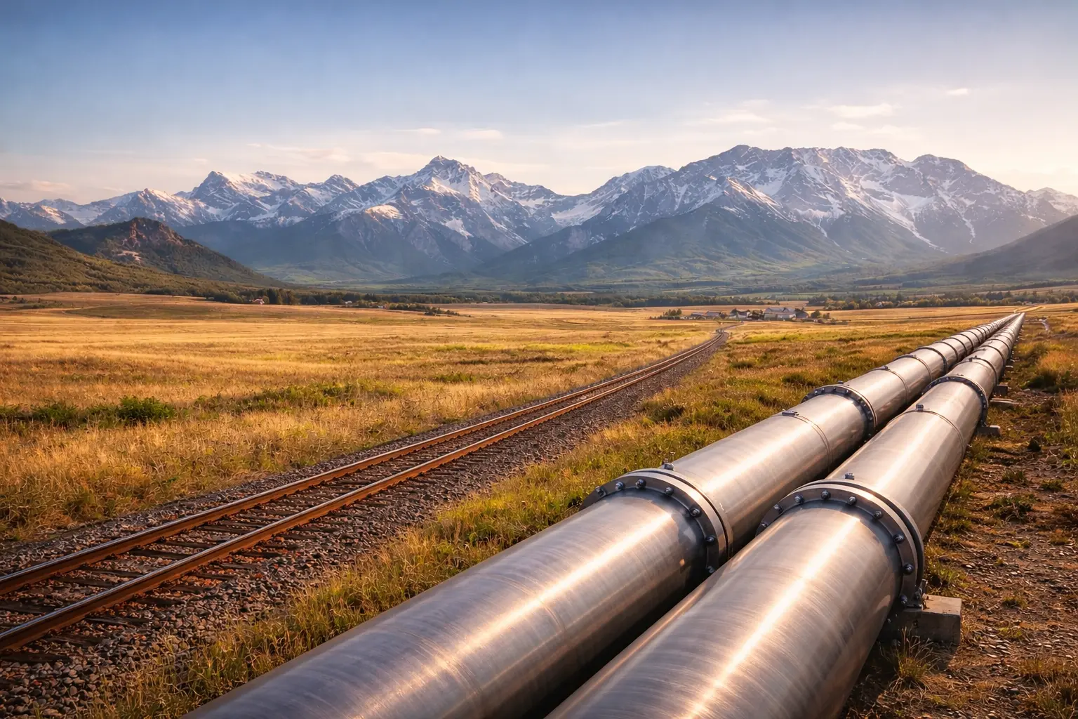
The NOVA Gas Transmission system

NOVA Gas Transmission Ltd (NGTL), owned by TC Energy, is the intra-Alberta gas transmission system. It is the backbone through which virtually all Alberta gas production moves before exiting the province.

Key facts about NGTL:

• Network extent: approximately 25,000 km of pipeline within Alberta
• Diameter range: 114 mm gathering laterals up to 914 mm (36-inch) main transmission lines
• Throughput: approximately 13–14 Bcf/d (billion cubic feet per day) at peak — roughly 370–400 million cubic metres per day
• Compressor stations: over 60 compressor stations maintaining system pressure
• AECO hub: the principal trading point for Alberta gas, located near Suffield in southeastern Alberta, where NGTL connects to export pipelines

NGTL is unusual among Canadian pipeline systems in that it serves both as a gathering system (collecting gas from thousands of wells) and as a transmission system (moving large volumes to export connections). This dual role means it operates simultaneously at multiple pressure levels across a vast geographic area.

The export corridors

Gas leaving Alberta via NGTL exits through several border connections:

Westbound — Pacific exports:

• Westcoast Energy / Spectra pipeline runs south from northeastern BC through BC to the U.S. border near Huntingdon/Sumas, connecting to the U.S. Pacific Northwest and California markets
• Alliance Pipeline runs from northeastern BC/Alberta to the Chicago area — a high-pressure, large-diameter (36-inch) line that moves approximately 1.6 Bcf/d in a single corridor

Southbound — U.S. Midwest and Rockies:

• TC Energy’s Canadian Mainline (formerly TransCanada) runs east from Alberta, but historically also fed U.S. interconnects via the Northern Border and Great Lakes pipeline systems
• Multiple small interconnects at the Alberta-Montana and Alberta-Saskatchewan-U.S. borders serve local Midwest markets

Eastbound — Canadian markets:

• TC Energy’s Canadian Mainline carries gas from Alberta east through Saskatchewan, Manitoba, Ontario, and Quebec — approximately 4,900 km to Montreal and connections to the Maritimes
• Flow on the Canadian Mainline has declined significantly as Ontario and Quebec shifted toward locally produced gas (from Appalachian plays via U.S. routes) and other energy sources — a structural change that has reduced Alberta’s eastward market share

The AECO-Henry Hub basis differential

The basis differential is the difference between the local gas price and the reference benchmark:

\[\text{Basis} = P_{\text{AECO}} - P_{\text{Henry Hub}}\]

This value is almost always negative — AECO trades at a discount to Henry Hub. The discount varies with season and pipeline capacity conditions, but has historically averaged CAD $1.00–$2.50/GJ, with occasional spikes to CAD $4–5/GJ during constraint events.

The discount exists because:

1. Transport cost: moving gas from AECO to Henry Hub costs money — approximately USD $0.50–$1.00/MMBtu in tariffs
2. Basis risk: shippers demand a discount to hold Alberta gas relative to a benchmark they can hedge on financial markets
3. Capacity constraints: when NGTL or export corridors are congested, Alberta gas cannot easily reach better-priced markets, and local oversupply depresses AECO

Understanding the basis differential quantitatively is the central economic lesson of Alberta’s gas transmission geography.

---

3. The Mathematical Model

The Weymouth equation for gas pipeline flow

For compressible gas flow in a pipeline, the Weymouth equation is a widely used approximation relating throughput to pressure, pipe geometry, and gas properties:

\[Q = 433.5 \cdot T_b \cdot \left(\frac{P_1^2 - P_2^2}{G \cdot T_f \cdot L \cdot Z}\right)^{0.5} \cdot D^{8/3} \cdot \frac{1}{P_b}\]

where in field units (common in the North American gas industry):

• $Q$ is gas flow rate (standard cubic feet per day, scf/d)
• $T_b$ is base temperature (520 °R = 60°F)
• $P_1$ is inlet pressure (psia)
• $P_2$ is outlet pressure (psia)
• $G$ is gas specific gravity (dimensionless; air = 1.0; natural gas $\approx$ 0.65)
• $T_f$ is mean flowing temperature (°R)
• $L$ is pipe length (miles)
• $Z$ is gas compressibility factor (dimensionless; $\approx$ 0.88–0.92 at typical pipeline conditions)
• $D$ is pipe internal diameter (inches)
• $P_b$ is base pressure (14.73 psia)

The key insight from this equation is the diameter exponent: flow rate scales as $D^{8/3} \approx D^{2.67}$. Doubling the diameter increases capacity by a factor of $2^{8/3} \approx 6.35$ — a far more powerful leverage than for liquid pipelines (where flow scales roughly as $D^{2.5}$ via Darcy-Weisbach). This is why gas transmission investments strongly favour large-diameter pipes.

Simplifying for understanding

Stripping the constants and rearranging, the Weymouth equation says:

\[Q \propto D^{8/3} \cdot \sqrt{\frac{P_1^2 - P_2^2}{G \cdot T \cdot L \cdot Z}}\]

Two proportionalities are immediately clear:

• Flow increases with the square root of the pressure differential $(P_1^2 - P_2^2)$: doubling the pressure ratio does not double the flow — it increases it by $\sqrt{2} \approx 1.41$
• Flow increases strongly with diameter ($D^{8/3}$): small increases in pipe diameter produce large gains in capacity

The basis differential as a transport cost

The minimum basis discount at which Alberta gas can reach Henry Hub is simply the all-in transport cost from AECO to Louisiana:

\[\text{Basis}_{\min} = -(T_{\text{NGTL}} + T_{\text{export}} + T_{\text{U.S.}})\]

where $T$ represents tariff segments in consistent units (CAD/GJ or USD/MMBtu). In practice, the market basis is at least as negative as the sum of tariffs; it widens further when capacity is constrained and Alberta gas cannot physically reach the destination.

Converting between common gas pricing units:

$$1 \text{ MMBtu} \approx 1.055 \text{ GJ} \approx 28.3 \text{ m}^3 \text{ (at standard conditions)}$$

\[P_{\text{CAD/GJ}} = P_{\text{USD/MMBtu}} \times \frac{1}{1.055} \times \frac{1}{\text{exchange rate (USD/CAD)}}\]

---

4. Worked Example by Hand

How much gas can a 36-inch Alliance Pipeline segment move?

Alliance Pipeline runs from northeastern BC/Alberta to Chicago — approximately 3,848 km (2,391 miles). Its design capacity is approximately 1.6 Bcf/d through a 36-inch (914 mm) pipeline.

Let us verify this with a simplified Weymouth calculation.

Given:

• $D = 36$ inches
• $L = 200$ miles (representative segment between compressor stations)
• $P_1 = 1,200$ psia (inlet, post-compression)
• $P_2 = 900$ psia (outlet, pre-next-compressor)
• $G = 0.65$ (Alberta gas specific gravity)
• $T_f = 540$ °R (80°F mean flowing temperature)
• $Z = 0.90$
• $T_b = 520$ °R, $P_b = 14.73$ psia

Step 1 — Compute pressure term:

\[P_1^2 - P_2^2 = 1{,}200^2 - 900^2 = 1{,}440{,}000 - 810{,}000 = 630{,}000 \text{ psia}^2\]

Step 2 — Compute the bracketed term:

\[\frac{P_1^2 - P_2^2}{G \cdot T_f \cdot L \cdot Z} = \frac{630{,}000}{0.65 \times 540 \times 200 \times 0.90} = \frac{630{,}000}{63{,}180} \approx 9.972\]

Step 3 — Square root:

\[\sqrt{9.972} \approx 3.158\]

Step 4 — Diameter term:

\[D^{8/3} = 36^{8/3}\]

$$36^{1/3} \approx 3.302 \qquad 36^{8/3} = 36^2 \times 36^{2/3} = 1{,}296 \times 10.90 \approx 14{,}126$$

Step 5 — Assemble:

\[Q = 433.5 \times \frac{520}{14.73} \times 3.158 \times 14{,}126\] \[Q = 433.5 \times 35.30 \times 3.158 \times 14{,}126\] \[Q \approx 433.5 \times 35.30 \times 44{,}614\] \[Q \approx 433.5 \times 1{,}574{,}874 \approx 682{,}707{,}000 \text{ scf/d} \approx 0.68 \text{ Bcf/d}\]

This is a single 200-mile segment between two compressor stations. With multiple compressor stations restoring pressure along Alliance’s full length, total system throughput of 1.6 Bcf/d is consistent with this per-segment calculation — each segment contributes independently to total system throughput.

Step 6 — Convert to economic terms:

At an AECO price of CAD $2.50/GJ:

$$1 \text{ Bcf} = 10^9 \text{ scf} \times 0.02832 \text{ m}^3/\text{scf} \times 0.03726 \text{ GJ/m}^3 \approx 1.055 \text{ PJ}$$

\[\text{Annual value of Alliance throughput} = 1.6 \text{ Bcf/d} \times 365 \times 1.055 \text{ PJ/Bcf} \times 1{,}000 \text{ GJ/PJ} \times \$2.50/\text{GJ}\] \[\approx 1.6 \times 365 \times 1{,}055 \times 2{,}500 \approx \$2.44 \text{ billion CAD/yr}\]

One pipeline, at AECO prices. At Henry Hub prices of USD $3.00/MMBtu (approximately CAD $4.35/GJ at current exchange rates), the same volume would be worth approximately CAD $3.52 billion/yr — the basis differential costs Alberta producers roughly CAD $1.1 billion/yr on Alliance throughput alone.

---

5. Computational Implementation

# Foundation Implementation
# Alberta natural gas pipeline: Weymouth flow, basis differential, market value

import math

# --- Unit conversions ---
SCF_TO_M3 = 0.028317        # standard cubic feet to cubic metres
M3_TO_GJ = 0.037260         # m³ of natural gas to GJ (approximate, WCSB gas)
MMBTU_TO_GJ = 1.05505       # MMBtu to GJ
BCF_TO_SCF = 1e9            # billion cubic feet to standard cubic feet

def weymouth_flow_scfd(inlet_psia: float,
                        outlet_psia: float,
                        diameter_in: float,
                        length_miles: float,
                        specific_gravity: float = 0.65,
                        temp_rankine: float = 540.0,
                        z_factor: float = 0.90,
                        T_base: float = 520.0,
                        P_base: float = 14.73) -> float:
    """
    Weymouth equation: gas flow rate in standard cubic feet per day.
    
    Parameters
    ----------
    inlet_psia      : upstream pressure (psia)
    outlet_psia     : downstream pressure (psia)
    diameter_in     : pipe internal diameter (inches)
    length_miles    : pipe segment length (miles)
    specific_gravity: gas specific gravity (air = 1.0)
    temp_rankine    : mean flowing temperature (°R)
    z_factor        : gas compressibility factor
    T_base          : base temperature (°R), standard = 520
    P_base          : base pressure (psia), standard = 14.73
    """
    pressure_term = (inlet_psia**2 - outlet_psia**2) / \
                    (specific_gravity * temp_rankine * length_miles * z_factor)
    diameter_term = diameter_in ** (8/3)
    return 433.5 * (T_base / P_base) * math.sqrt(pressure_term) * diameter_term

def bcfd_from_scfd(scfd: float) -> float:
    """Convert scf/d to Bcf/d."""
    return scfd / BCF_TO_SCF

def annual_value_cad(bcfd: float, price_cad_gj: float) -> float:
    """Annual market value of a gas volume in CAD."""
    m3_per_day = bcfd * BCF_TO_SCF * SCF_TO_M3
    gj_per_day = m3_per_day * M3_TO_GJ
    return gj_per_day * 365 * price_cad_gj

def basis_cost_cad_yr(bcfd: float,
                       aeco_cad_gj: float,
                       henry_hub_usd_mmbtu: float,
                       exchange_rate: float = 0.73) -> float:
    """Annual revenue lost to AECO-Henry Hub basis differential."""
    henry_cad_gj = (henry_hub_usd_mmbtu / MMBTU_TO_GJ) / exchange_rate
    basis_cad_gj = aeco_cad_gj - henry_cad_gj
    m3_per_day = bcfd * BCF_TO_SCF * SCF_TO_M3
    gj_per_day = m3_per_day * M3_TO_GJ
    return basis_cad_gj * gj_per_day * 365  # negative = revenue loss

# --- Alberta export pipeline inventory ---
PIPELINES = {
    "Alliance Pipeline":           {"bcfd": 1.60, "diameter_in": 36, "length_km": 3848, "market": "Chicago / U.S. Midwest"},
    "TC Mainline (eastbound)":     {"bcfd": 4.20, "diameter_in": 42, "length_km": 4900, "market": "Ontario / Quebec / Maritimes"},
    "Westcoast / Spectra":         {"bcfd": 2.80, "diameter_in": 36, "length_km": 1200, "market": "Pacific Northwest / California"},
    "TCPL to U.S. Midwest":        {"bcfd": 1.50, "diameter_in": 36, "length_km": 800,  "market": "U.S. Midwest (various)"},
    "Foothills (to U.S. Rockies)": {"bcfd": 0.80, "diameter_in": 30, "length_km": 1000, "market": "U.S. Rockies / California"},
}

AECO_PRICE = 2.50       # CAD/GJ — approximate 2024 average
HENRY_HUB_PRICE = 2.80  # USD/MMBtu — approximate 2024 average
EXCHANGE_RATE = 0.73    # USD/CAD

print("=== Alberta Natural Gas Export Pipeline Network ===\n")
print(f"{'Pipeline':<35} {'Capacity':>10} {'Market'}")
print(f"  {'(Bcf/d)':>33}")
print("-" * 75)
total_bcfd = 0
for name, p in PIPELINES.items():
    print(f"{name:<35} {p['bcfd']:>10.2f}  {p['market']}")
    total_bcfd += p["bcfd"]
print("-" * 75)
print(f"{'TOTAL EXPORT CAPACITY':<35} {total_bcfd:>10.2f}")

print(f"\n=== Weymouth Verification: Alliance Pipeline ===\n")
q_scfd = weymouth_flow_scfd(
    inlet_psia=1200, outlet_psia=900,
    diameter_in=36, length_miles=124,  # ~200 km segment
    specific_gravity=0.65, temp_rankine=540, z_factor=0.90
)
q_bcfd = bcfd_from_scfd(q_scfd)
print(f"  Segment (200 km, 36-in, 1200→900 psia):")
print(f"  Q = {q_scfd:,.0f} scf/d = {q_bcfd:.3f} Bcf/d per segment")

print(f"\n=== AECO vs Henry Hub: Annual Revenue Comparison ===\n")
print(f"  AECO price    : CAD ${AECO_PRICE:.2f}/GJ")
henry_cad_gj = (HENRY_HUB_PRICE / MMBTU_TO_GJ) / EXCHANGE_RATE
print(f"  Henry Hub     : USD ${HENRY_HUB_PRICE:.2f}/MMBtu "
      f"= CAD ${henry_cad_gj:.2f}/GJ (at {EXCHANGE_RATE} CAD/USD)")
print(f"  Basis (AECO − HH): CAD ${AECO_PRICE - henry_cad_gj:.2f}/GJ\n")

total_basis_loss = 0
for name, p in PIPELINES.items():
    val_aeco = annual_value_cad(p["bcfd"], AECO_PRICE)
    basis_loss = basis_cost_cad_yr(p["bcfd"], AECO_PRICE, HENRY_HUB_PRICE, EXCHANGE_RATE)
    total_basis_loss += basis_loss
    print(f"  {name:<35}")
    print(f"    Value at AECO    : CAD ${val_aeco/1e9:.2f}B/yr")
    print(f"    Basis cost       : CAD ${-basis_loss/1e6:.0f}M/yr\n")

print(f"  Total annual basis cost across all export corridors:")
print(f"    CAD ${-total_basis_loss/1e9:.2f} billion/year")

Professional Implementation

# Professional Implementation
# Gas pipeline network: multi-segment Weymouth, compressor energy, basis analysis

import math
from dataclasses import dataclass, field
from typing import Optional

# Physical constants
R_GAS = 8.314       # J/(mol·K)
MW_AIR = 28.97      # g/mol
SCF_TO_M3 = 0.028317
M3_TO_GJ = 0.03726
MMBTU_TO_GJ = 1.05505
BCF_TO_SCF = 1e9
HP_TO_KW = 0.7457

@dataclass
class PipeSegment:
    """A single pipeline segment between compressor stations."""
    name: str
    diameter_in: float
    length_miles: float
    inlet_psia: float
    outlet_psia: float
    specific_gravity: float = 0.65
    temp_rankine: float = 540.0
    z_factor: float = 0.90

    def flow_scfd(self) -> float:
        """Weymouth equation flow rate (scf/d)."""
        P_sq_diff = self.inlet_psia**2 - self.outlet_psia**2
        denom = (self.specific_gravity * self.temp_rankine
                 * self.length_miles * self.z_factor)
        return (433.5 * (520 / 14.73)
                * math.sqrt(P_sq_diff / denom)
                * self.diameter_in ** (8/3))

    def flow_bcfd(self) -> float:
        return self.flow_scfd() / BCF_TO_SCF

    def flow_m3_per_day(self) -> float:
        return self.flow_scfd() * SCF_TO_M3

    def compressor_power_hp(self,
                             efficiency: float = 0.80,
                             gamma: float = 1.27) -> float:
        """
        Approximate compressor power to re-raise outlet to inlet pressure.
        Uses isentropic compression work formula.
        """
        r = self.inlet_psia / self.outlet_psia  # compression ratio
        q_m3s = self.flow_m3_per_day() / 86400
        # Inlet density (ideal gas approximation)
        rho = (self.outlet_psia * 6894.76) / (self.z_factor * 287 * (self.temp_rankine / 1.8))
        w_isentropic = ((gamma / (gamma - 1))
                        * (self.outlet_psia * 6894.76 / rho)
                        * (r ** ((gamma - 1) / gamma) - 1))
        power_w = q_m3s * rho * w_isentropic / efficiency
        return power_w / 745.7  # convert to horsepower


@dataclass
class GasPipeline:
    """Multi-segment gas pipeline with compressor stations."""
    name: str
    market: str
    segments: list[PipeSegment] = field(default_factory=list)
    commissioned_year: Optional[int] = None

    def capacity_bcfd(self) -> float:
        """Minimum segment flow = system capacity (series flow)."""
        if not self.segments:
            return 0.0
        return min(s.flow_bcfd() for s in self.segments)

    def total_compressor_power_hp(self) -> float:
        return sum(s.compressor_power_hp() for s in self.segments)

    def annual_gj(self) -> float:
        m3_day = self.capacity_bcfd() * BCF_TO_SCF * SCF_TO_M3
        return m3_day * 365 * M3_TO_GJ

    def annual_revenue_cad(self, price_cad_gj: float) -> float:
        return self.annual_gj() * price_cad_gj


@dataclass
class GasMarketAnalysis:
    pipelines: list[GasPipeline]
    aeco_cad_gj: float
    henry_hub_usd_mmbtu: float
    exchange_rate_usd_cad: float = 0.73

    @property
    def henry_hub_cad_gj(self) -> float:
        return (self.henry_hub_usd_mmbtu / MMBTU_TO_GJ) / self.exchange_rate_usd_cad

    @property
    def basis_cad_gj(self) -> float:
        return self.aeco_cad_gj - self.henry_hub_cad_gj

    @property
    def total_capacity_bcfd(self) -> float:
        return sum(p.capacity_bcfd() for p in self.pipelines)

    def annual_basis_cost_cad(self) -> float:
        total_gj = sum(p.annual_gj() for p in self.pipelines)
        return total_gj * self.basis_cad_gj  # negative = cost

    def report(self):
        print(f"\n{'='*68}")
        print(f"  Alberta Gas Export Market Analysis")
        print(f"{'='*68}")
        print(f"\n  Price benchmarks:")
        print(f"    AECO (Alberta)  : CAD ${self.aeco_cad_gj:.2f}/GJ")
        print(f"    Henry Hub (LA)  : USD ${self.henry_hub_usd_mmbtu:.2f}/MMBtu"
              f" = CAD ${self.henry_hub_cad_gj:.2f}/GJ")
        print(f"    Basis           : CAD ${self.basis_cad_gj:.2f}/GJ")

        print(f"\n  {'Pipeline':<32} {'Cap (Bcf/d)':>11} {'Rev @AECO':>13} {'Basis cost':>12}")
        print(f"  {'-'*70}")

        total_rev = 0
        total_basis = 0
        for p in self.pipelines:
            cap = p.capacity_bcfd()
            rev = p.annual_revenue_cad(self.aeco_cad_gj)
            basis = p.annual_gj() * self.basis_cad_gj
            total_rev += rev
            total_basis += basis
            print(f"  {p.name:<32} {cap:>11.2f} "
                  f"${rev/1e9:>9.2f}B/yr "
                  f"${-basis/1e6:>8.0f}M/yr")

        print(f"  {'-'*70}")
        print(f"  {'TOTAL':<32} {self.total_capacity_bcfd:>11.2f} "
              f"${total_rev/1e9:>9.2f}B/yr "
              f"${-total_basis/1e9:>8.2f}B/yr")
        print(f"\n  Annual basis cost (AECO discount vs Henry Hub):")
        print(f"    CAD ${-self.annual_basis_cost_cad()/1e9:.2f} billion/year")


# --- Build the pipeline segments ---
# Alliance — representative 200-km segments
alliance_segs = [
    PipeSegment("Alliance S1", 36, 124, 1200, 900),
    PipeSegment("Alliance S2", 36, 124, 1200, 900),
    PipeSegment("Alliance S3", 36, 124, 1200, 900),
]
alliance = GasPipeline("Alliance Pipeline", "Chicago / Midwest",
                        alliance_segs, 2000)

# TC Mainline — larger diameter, longer segments
mainline_segs = [
    PipeSegment("TC ML S1", 42, 150, 1200, 850),
    PipeSegment("TC ML S2", 42, 150, 1200, 850),
    PipeSegment("TC ML S3", 42, 150, 1200, 850),
]
tc_mainline = GasPipeline("TC Canadian Mainline", "Ontario / Quebec",
                           mainline_segs, 1958)

westcoast_segs = [
    PipeSegment("Westcoast S1", 36, 100, 1100, 850),
    PipeSegment("Westcoast S2", 36, 100, 1100, 850),
]
westcoast = GasPipeline("Westcoast / Spectra", "Pacific NW / California",
                         westcoast_segs, 1957)

analysis = GasMarketAnalysis(
    pipelines=[alliance, tc_mainline, westcoast],
    aeco_cad_gj=2.50,
    henry_hub_usd_mmbtu=2.80,
    exchange_rate_usd_cad=0.73
)
analysis.report()

# --- Compressor power summary ---
print(f"\n  Compressor power estimates:")
for p in analysis.pipelines:
    hp = p.total_compressor_power_hp()
    print(f"    {p.name:<32}: {hp:>10,.0f} hp  ({hp * HP_TO_KW / 1000:.1f} MW)")

---

6. Visualization

Figure 1 — Alberta Gas Export Capacity by Corridor

Figure 2 — AECO vs Henry Hub: Historical Price Comparison

Figure 3 — Weymouth Equation: Diameter vs. Flow Capacity

Figure 4 — Annual Basis Cost by Export Corridor

Figure 5 — NGTL System Extent and Export Connections

---

7. Interpretation

Alberta is the dominant Canadian gas producer — but not the price setter

Alberta’s approximately 70% share of Canadian natural gas production is a function of geology: the Western Canadian Sedimentary Basin contains the Montney, Duvernay, and Deep Basin plays, which together represent some of the largest tight gas and shale gas resources in North America. Production has grown substantially since 2016 as horizontal drilling and hydraulic fracturing unlocked the Montney in particular — a play straddling the Alberta-BC border with recoverable resource estimates comparable to major U.S. shale plays.

But volume does not confer price-setting power when the physical constraints of the pipeline system create a price discount at the production hub. AECO is the price Alberta producers actually receive. Henry Hub is the price Alberta gas is worth at the North American clearing market. The gap between them — the basis differential — is the geographic tax that distance and pipeline capacity impose on every GJ Alberta produces.

The basis differential is not constant — it is a signal

The historical data in Figure 2 show that the basis differential widens sharply during constraint events. In 2018, AECO collapsed to CAD $1.10/GJ while Henry Hub traded near CAD $4.20/GJ — a basis of nearly -$3.10/GJ. This was not a policy failure or a market manipulation; it was the result of NGTL running near capacity during a period of rapid Montney production growth, while export pipeline additions lagged. Gas that could not leave Alberta accumulated at AECO and depressed the price.

The 2018 basis crisis prompted TC Energy’s NGTL expansion program and new export interconnects. The basis subsequently narrowed. This sequence — production growth outpacing infrastructure, basis widening, investment responding, basis recovering — is the normal dynamic of a pipeline-constrained gas market. It is also a quantitatively observable phenomenon that the Weymouth equation and basis arithmetic can model in advance.

The TC Canadian Mainline’s decline is structural

The TC Mainline runs 4,900 km from Alberta to Quebec — the longest gas pipeline in the world by some measures. It was once Alberta’s primary export artery. In recent decades, its eastward utilization has declined significantly as Ontario and Quebec natural gas demand flattened, as those provinces began receiving Appalachian gas via U.S. pipelines, and as fuel switching reduced industrial gas demand. TC Energy’s 2024 regulatory proceedings around the Mainline’s contracting model reflect this structural overcapacity. Alberta’s eastward market has shrunk; the pipe remains.

LNG export: the missing Pacific corridor

The one major export corridor that does not yet exist is LNG export from the British Columbia coast. LNG Canada’s Kitimat terminal — the first phase of which entered commissioning in 2024 — will take up to 1.8 Bcf/d of Coastal GasLink (from northeastern BC Montney) and export it as liquefied natural gas to Asian markets. For Alberta producers, LNG Canada matters because it tightens the Montney supply market that supplies both BC and Alberta pipelines. A fully contracted LNG Canada would remove supply from the AECO market, putting upward pressure on AECO prices — a meaningful basis improvement for Alberta producers even though the LNG terminal itself is in BC, not Alberta.

---

8. What Could Go Wrong?

Weymouth equation limitations

The Weymouth equation is an empirical approximation suited for turbulent flow in large-diameter gas pipelines. It overpredicts capacity at lower Reynolds numbers and does not account for:

• Elevation changes: the NGTL system crosses varied terrain; the hydrostatic pressure of gas columns in hilly terrain affects actual flow
• Water and liquid content: entrained liquids dramatically increase friction and reduce throughput
• Temperature variations: gas temperature changes with ambient conditions and compression heat; the fixed $T_f$ assumption is a simplification

For detailed engineering design, the AGA (American Gas Association) full turbulent flow equations and numerical simulation (TGNET, Synergi) replace the Weymouth approximation.

Basis differential volatility

The annual average basis figures used here smooth over significant intra-year variation. AECO can trade at a premium to Henry Hub briefly during cold spells when Alberta demand spikes. It can collapse to near zero or negative values during spring maintenance windows when production continues but demand falls and pipeline space is occupied by maintenance scheduling. Producers typically hedge through financial basis swaps, but perfect hedging is expensive.

LNG Canada timing and volumes

The LNG Canada capacity figure here is based on Phase 1 design capacity. The timing of full commissioning, Phase 2 expansion decisions, and the impact on AECO pricing all remain uncertain as of early 2026.

---

9. Summary

Alberta’s natural gas pipeline system is built around the NOVA Gas Transmission system — 25,000 km of intra-provincial gathering and transmission — connected to five main export corridors serving eastern Canada, the U.S. Midwest, the U.S. Pacific Northwest and California, and the U.S. Rockies.

The key quantitative facts:

• Total export capacity: approximately 10.9 Bcf/d across all corridors, against provincial production of 15–17 Bcf/d (remainder consumed in-province or stored)
• AECO-Henry Hub basis: historically CAD -$1.00 to -$3.10/GJ; at current conditions approximately -$1.15/GJ, representing roughly CAD $1.5 billion/year in revenue foregone across major corridors
• Weymouth diameter leverage: a 42-inch pipe carries 5.16 times the flow of a 24-inch pipe at identical pressure conditions — the single most powerful engineering lever in gas transmission
• TC Mainline decline: the 4,900 km eastward corridor is structurally underutilized as eastern Canadian markets diversify supply
• LNG Canada represents the first significant new market access for WCSB gas producers in decades — a structural basis improvement if Phase 2 proceeds

Geography sets the cost of distance. The Weymouth equation quantifies it. The basis differential prices it.

---

Math Refresher

Gas volume units and conversions

Natural gas volumes are measured at standard conditions (typically 15°C and 101.325 kPa in Canada; 60°F and 14.73 psia in the U.S.). This standardization is necessary because gas is compressible — the same mass of gas occupies different volumes at different pressures.

Unit	Equivalent
1 thousand cubic feet (Mcf)	28.32 m³
1 million cubic feet (MMcf)	28,317 m³
1 billion cubic feet (Bcf)	28.32 million m³
1 MMBtu	1.05505 GJ
1 m³ natural gas	~0.0373 GJ (WCSB typical)

Reading the Weymouth exponent

The key result $Q \propto D^{8/3}$ comes from the pipe cross-section ($A \propto D^2$) combined with the friction term, which for the Weymouth equation yields $D^{2/3}$ additional leverage over the Darcy-Weisbach treatment. The total $D^{8/3} = D^{2+2/3}$ means each inch of additional diameter buys disproportionate capacity — which is why 36-inch and 42-inch pipelines dominate long-distance gas transmission.

---

Sources and Data Notes

Source	Used For
Canada Energy Regulator, Natural Gas Market Assessment (2024)	NGTL throughput, export capacity, market context
TC Energy, NGTL System Overview and Regulatory Filings (2024)	Network extent, compressor count, capacity
Canada Energy Regulator, AECO Price Data (2015–2024)	Historical AECO prices
U.S. Energy Information Administration, Henry Hub Price Data	Historical Henry Hub prices
Alliance Pipeline, System Overview (2023)	Capacity, route, diameter
LNG Canada, Project Update (2024)	Kitimat terminal status, capacity
Weymouth, T.R. (1912), Transactions of the ASCE	Original Weymouth equation derivation
Menon, E.S., Gas Pipeline Hydraulics (2005)	Weymouth equation field-unit form and application

AECO and Henry Hub prices are calendar-year averages and are approximate. Basis differential calculations are illustrative. All throughput figures are nameplate capacity; actual throughput varies with nominations and operating conditions.

---

References

Alberta Government. n.d. Natural Gas Price Variables. Edmonton: Government of Alberta. https://www.alberta.ca/natural-gas-price-variables

Canada Energy Regulator. 2024. Market Snapshot: Exploring Canada’s Future in LNG Exports. Calgary: CER. https://www.cer-rec.gc.ca/en/data-analysis/energy-markets/market-snapshots/2024/market-snapshot-exploring-canadas-future-in-lng-exports.html

Canada Energy Regulator. 2024. Market Snapshot: Western Canada’s Natural Gas Export Pipelines Continued to See High Utilization in 2023. Calgary: CER. https://www.cer-rec.gc.ca/en/data-analysis/energy-markets/market-snapshots/2024/market-snapshot-western-canadas-natural-gas-export-pipelines-continued-to-see-high-utilization-in-2023.html

Canada Energy Regulator. 2024. Pipeline Profiles: NOVA Gas Transmission Ltd. (NGTL). Calgary: CER. https://www.cer-rec.gc.ca/en/data-analysis/facilities-we-regulate/pipeline-profiles/natural-gas/pipeline-profiles-ngtl.html

Canada Energy Regulator. 2024. Pipeline Profiles: TC Canadian Mainline. Calgary: CER. https://www.cer-rec.gc.ca/en/data-analysis/facilities-we-regulate/pipeline-profiles/natural-gas/pipeline-profiles-transcanadas-canadian-mainline.html

Canada Energy Regulator. 2024. Pipeline Profiles: Alliance. Calgary: CER. https://apps.cer-rec.gc.ca/PPS/en/pipeline-profiles/alliance

Canada Energy Regulator. 2025. Market Snapshot: Canadian Natural Gas Production Continues to Reach Record Levels. Calgary: CER. https://www.cer-rec.gc.ca/en/data-analysis/energy-markets/market-snapshots/2025/market-snapshot-canadian-natural-gas-production-continues-to-reach-record-levels.html

LNG Canada. 2024. “LNG Canada 2024 Fall Update.” Kitimat: LNG Canada. https://www.lngcanada.ca/news/lng-canada-2024-fall-update/

Menon, E. Shashi. 2005. Gas Pipeline Hydraulics. Boca Raton: CRC Press. https://www.taylorfrancis.com/books/mono/10.1201/9781420038224/gas-pipeline-hydraulics-shashi-menon

Pembina Pipeline Corporation. 2024. Alliance Pipeline. Calgary: Pembina. https://www.pembina.com/operations/pipelines/alliance-pipeline

TC Energy. 2024. Canadian Mainline. Calgary: TC Energy. https://www.tcenergy.com/operations/natural-gas/canadian-mainline/

TC Energy. 2024. NGTL System. Calgary: TC Energy. https://www.tcenergy.com/operations/natural-gas/ngtl-system/

U.S. Energy Information Administration. 2021. “Higher Western Canada Spot Prices Limit U.S. Natural Gas Imports from Canada.” Washington, DC: EIA. https://www.eia.gov/todayinenergy/detail.php?id=44175

Weymouth, Thomas R. 1912. “Problems in Natural Gas Engineering.” Transactions of the American Society of Mechanical Engineers 34: 185–231. (No public URL available — published before digital archiving; cited via Menon 2005.)

---